9.7 Linear regression diagnostics

Finally, what if we have a continuous explanatory variable and a continuous response that necessitates use of linear regression or ANCOVA?

We use the same approach (whoa, that’s sweet, huh?). Here, let’s fit and assess a model that predicts the length of Stay in turtle rehab based on the hook Width that caught them in the first place.

# Fit the model
fit_width <- lm( Stay ~ Width, data = turtles)

# Now plot the residuals
ggplot(fit_width, aes(x = .fitted, y = .resid, color = Width)) + 
  geom_point() +
  xlab("Hook width") + 
  ylab(expression(paste(epsilon)))

Bleh. As with our example above, we can see that we clearly fail the assumption that the residuals are normally distributed with a mean of zero! It also looks like the residual error increases with increasing hook width, which means our observations are also not independent. This specific type of non-independence is called heteroscedasticity. That’s a real word.

Let’s see if our new toy, the log-transformation can help us here:

# Fit the model
log_fit_width <- lm( log(Stay) ~ Width, data = turtles)

# Now plot the residuals
ggplot(log_fit_width, aes(x = .fitted, y = .resid, color = Width)) + 
  geom_point() +
  xlab("Hook width") + 
  ylab(expression(paste(epsilon)))

Wow, that actually looks a whole lot better! There are still a couple of data points flying high that we would want to investigate further in this data set, but the pukey feeling in my stomach is slowly subsiding here.

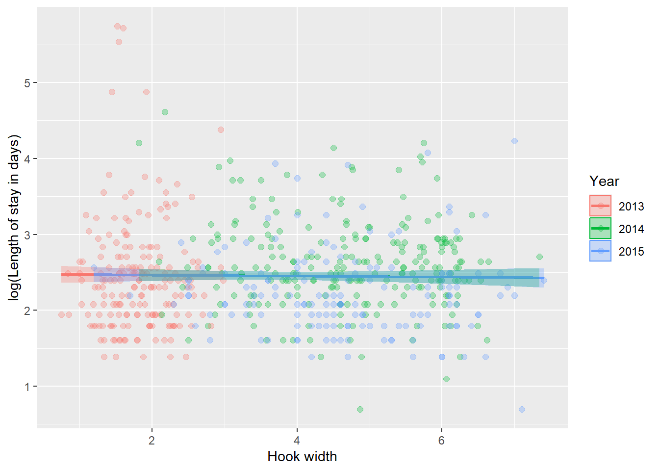
And remember, if you really want to see how your model fits the data, you could always plot the predictions over the raw data:

# Need to get rid of a couple NA values
turts <- subset(turtles, !is.na(Width))

log_fit_width <- lm( log(Stay) ~ Width, data = turts)
turt_pred <- cbind(turts, predict(log_fit_width, interval = 'confidence'))

ggplot(turt_pred, aes(x = Width, y = log(Stay), color = Year, fill = Year)) +
  geom_point(alpha = 0.3, size = 2) +
  geom_line(aes(y = fit), size = 1) +
  geom_ribbon(aes(ymin = lwr, ymax = upr, color = NULL), alpha = .3) +
  xlab("Hook width") +
  ylab("log(Length of stay in days)")

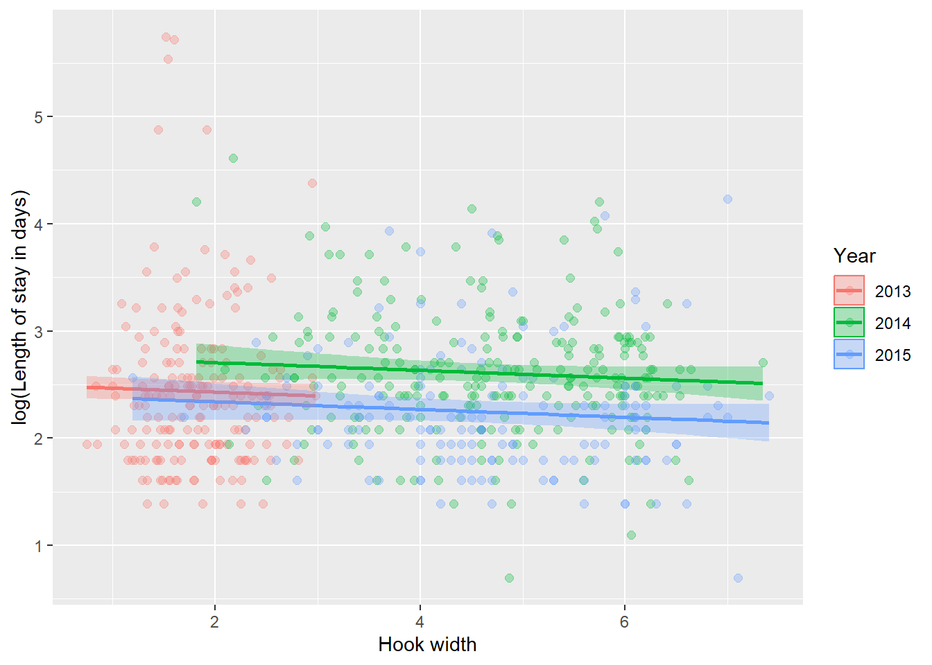
Surely this plot alone is evidence enough that we need to investigate confounding between hook Width and Year in any further investigation into this data set! Maybe with an ANCOVA?

# Need to get rid of a couple NA values
turts <- subset(turtles, !is.na(Width))

log_fit_width <- lm( log(Stay) ~ Year + Width, data = turts)
turt_pred <- cbind(turts, predict(log_fit_width, interval = 'confidence'))

ggplot(turt_pred, 
       aes(x = Width, y = log(Stay), color = Year, fill = Year)) +
  geom_point(alpha = 0.3, size = 2) +
  geom_line(aes(y = fit), size = 1) +
  geom_ribbon(aes(ymin = lwr, ymax = upr, color = NULL), alpha = .3) +
  xlab("Hook width") +
  ylab("log(Length of stay in days)")

Holy crap…three lines. Where did the other two come from? Keep reading to find out in Chapter 10.

Notice that we still have not looked at the results of any of these models.