20.2 Logistic regression {#20-logistic}

For our first example this week, we will use the choice data from a couple weeks ago that we used to demonstrate binomial logistic regression. This time, we will add in a random intercept term that will allow us to account for repeated observations within a year. This has two implications: 1) it accounts for the fact that the years in which we conducted this study are random samples from a larger, unobserved population, and 2) it accounts for the heterogeneity of variance that theoretically might occur as a result of taking multiple, and variable, numbers of measurements within a given year- thereby reducing the overall error of the model and our associated parameter estimates (in theory).

##   path year hatchery length mass date flow
## 1    0 2010        1    176   57  118  345
## 2    0 2005        1    205  101  128 1093
## 3    0 2010        1    180   56  118  345
## 4    0 2010        1    193   74  118  345
## 5    0 2005        1    189   76  128 1093
## 6    0 2010        1    180   65  118  345

20.2.1 Data Explanation {#20-logistic-data}

These data are from a study that examined factors affecting path choice by wild and hatchery-reared endangered Atlantic salmon smolts during seaward migration in the Penobscot River, Maine. State, local, and federal fishery managers were interested in understanding what factors affected migratory routing through the lower river because there were different numbers of dams, with different estimated smolt mortality rates, on either side of a large island hydropower project in this system. If managers could understand factors influencing migratory route, they might be able to manipulate flows, stocking dates, and dam operation to improve survival of these endangered fish. Furthermore, the results of the study were used to predict the effects of dam removal, and hydropower re-allocation in the lower river on population-level consequences for these fish. Please see the <08_glm_logisticRegression>logistic regression module for a complete explanation of the data.

20.2.2 Data analysis {#20-logistic-analysis}

We are going to use the 1/0 binary data to estimate the effects of a number of covariates of interest on the probability that an individual fish used the Stillwater Branch for migration in each year of this study using logistic regression.

Since we are not interested in the linear trend in the use of the Stillwater Branch through time, we need to convert year to factor. This is the same as if we wanted to use this as a fixed effect in the model as we did in Chapter 12.4 when we last worked with these data.

choice$year <- as.factor(choice$year)

Rather than run all of the models that we ran in Chapter 17 I am just going to run the best one because these models take a little longer to run than the non-hierarchical formulations.

best_mod <- stan_glmer(path ~ (1 | year) + flow, family = binomial, data = choice)

20.2.3 Predictions {#20-logistic-preds}

Finally, we can use these models to make predictions.

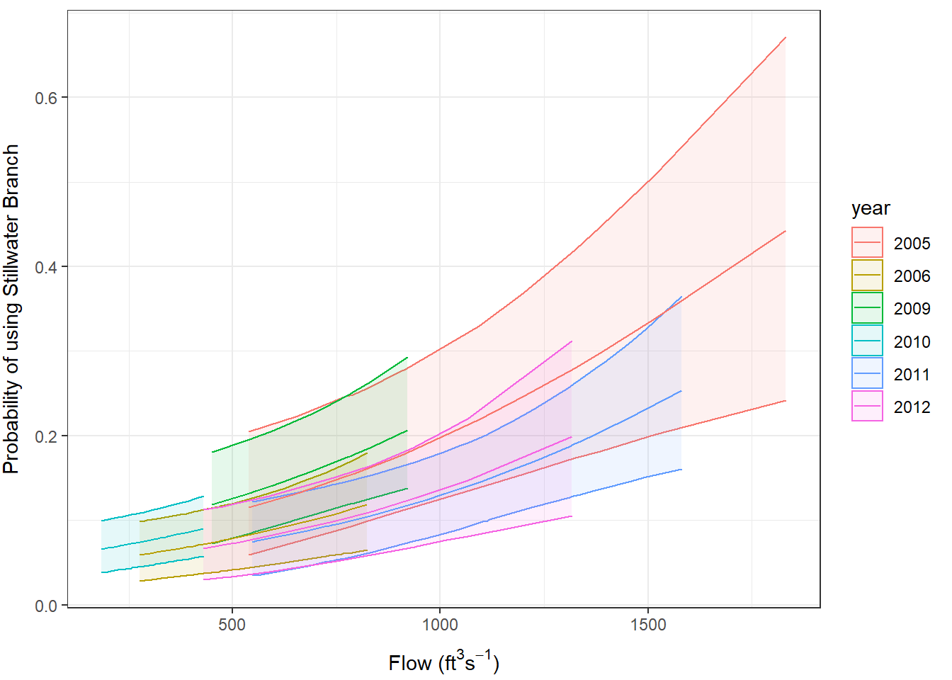
This is a little funky for binomial stan_glmer() models in rstanarm right now because the prevailing wisdom is to predict outcomes from hierarchical models fit with rstanarm. For binomial models, this means the output of posterior_predict() is ones and zeroes, which is not too terribly useful for visualizing the model results for those less mathematically inclined. Instead, we would like to see how probability of using Stillwater Branch changes in relation to our explanatory variables.

We will create a quick function using some of the rstanarm internals based on this example. My guess is that this will probably be implemented in the package by the next time I teach the class and edit this book.

predicted_prob <- function(fit) {
  dat <- rstanarm:::pp_data(fit)
  eta <- rstanarm:::pp_eta(fit, dat)$eta
  invlogit(eta) # inverse-logit 
}

Now, we can make predictions about the probability of using Stillwater Branch on each row of our observed data (or new data if we want!) using this function.

pred_matrix <- predicted_prob(best_mod)

The result is a matrix with 4,000 rows (1,000 iterations x 4 chains) of predicted probability of using the Stillwater Branch for each fish (row) from our original data. That is, the rows in original data correspond to the columns in pred_matrix. We can summarize this object the same way we did in Chapter 19 and add the descriptive statistics to the original data set for easy visualization. Note that we do not need to invert the logit because we already did that inside the predict_prob() function we created.

# Calculate descriptive statistics for predicted probability
# of using Stillwater Branch
fit <- apply(pred_matrix, 2, mean)
lwr <- apply(pred_matrix, 2, quantile, 0.025)
upr <- apply(pred_matrix, 2, quantile, 0.975)

# Smoosh them back together with the original data for plotting
choice_preds <- data.frame(choice, fit, lwr, upr)

And now, it is all over but the plotting:

ggplot(choice_preds, aes(x = flow, y = fit, color = year, fill = year)) +
  geom_ribbon(aes(xmax = flow, ymin = lwr, ymax = upr), alpha = 0.10) +
  geom_line() +
  xlab(expression(paste("Flow (ft"^3,"s"^-1, ")"))) +
  ylab("Probability of using Stillwater Branch") +
  theme_bw() +
  theme(
    axis.title.x = element_text(vjust = -1),
    axis.title.y = element_text(vjust = 3)
  )