3.6 Data simulation

The point of simulation is usually to account for uncertainty in some process (i.e. we could just pick a single value if we knew it). This is almost always done based on probability. There are a number of ways we could do this. One is by drawing from some probability distribution that we have described, and the other is by randomly sampling data that we already have.

3.6.1 Random sub-samples from a dataset

Let’s say we want to take random samples from our huge data set so we can fit models to a subset of data and then use the rest of our data for model validation in weeks to come.

We have around 17,000 observations in the am_shad data set. But, what if we wanted to know what it would look like if we only had 100 samples from the same population?

First, tell R how many samples you want.

n_samples <- 100

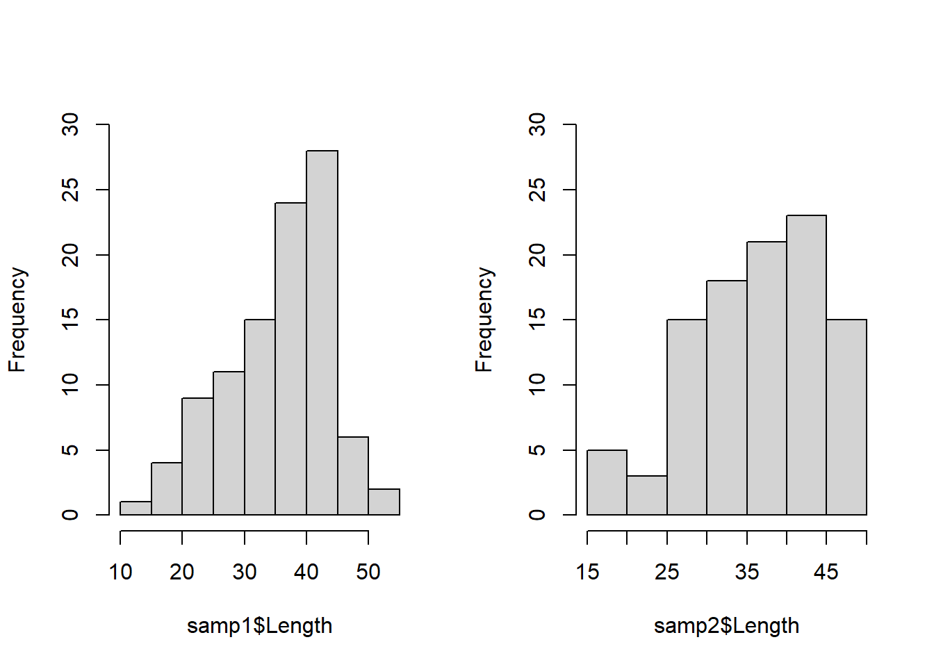
Now let’s take two samples of 100 fish from our dataframe to see how they compare:

# Randomly sample 100 rows of data from our data frame two different
# times to see the differences
samp1 <- am_shad[sample(nrow(am_shad), size = n_samples, replace = FALSE), ]
samp2 <- am_shad[sample(nrow(am_shad), size = n_samples, replace = FALSE), ]

# We can look at them with our histograms
par(mfrow = c(1, 2))
hist(samp1$Length, main = "", ylim = c(0, 30))
hist(samp2$Length, main = "", ylim = c(0, 30))

*If you are struggling to get your plotting window back to “normal” after this, you can either click the broom button in your “Plots” window, or you can run the following code for now:

3.6.2 Stochastic simulation

Now, instead of sampling our data let’s say we have some distribution from which we would like sample. So, let’s make a distribution.

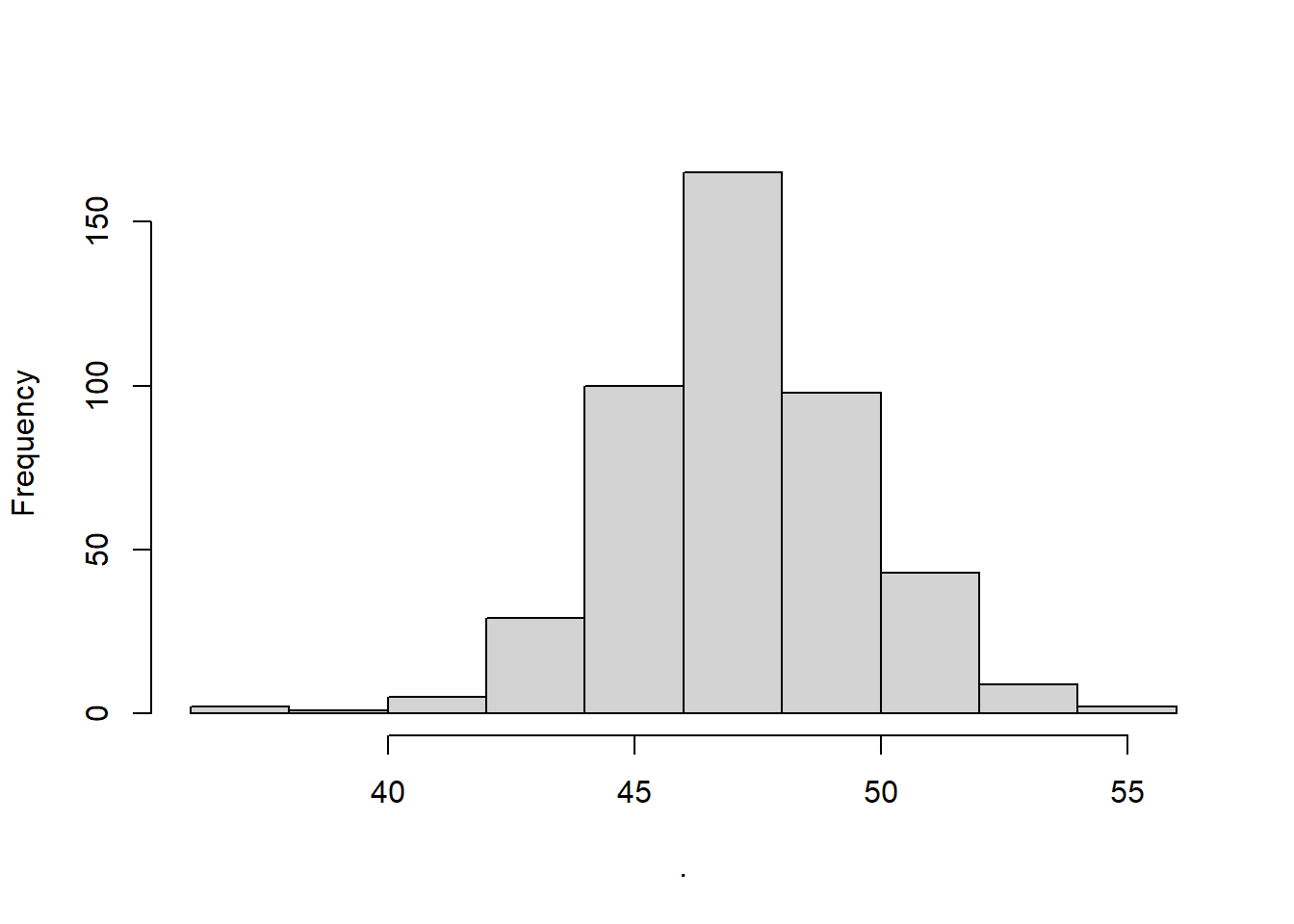
We will start with the normal, and we can move into others when we talk about probability distributions and sample statistics in Chapter 5. For this, we will use the distribution of American shad lengths for age-6 females because it approximates a normal distribution. We will calculate the mean and sd because those are the parameters of the normal distribution.

Start by looking at the size distribution for age 6 females. We use the tidy workflow here with really awful default graphics (more to come in Chapter 4), but we add two arguments to our subset call. We want to select only the variable Length from am_shad, and we want to drop all other information so we can send the output straight to the hist() function as a vector.

am_shad %>%
  subset(Age == 6 & Sex == "R", select='Length', drop=TRUE) %>%
   hist(main = "")

Now, let’s calculate the mean and sd of Length for age 6 females.

# Calculate the mean Length 
x_bar <- am_shad %>%
  subset(Age == 6 & Sex == "R", select='Length', drop=TRUE) %>%
  mean

# Calculate standard deviation of Length
sigma <- am_shad %>%
  subset(Age == 6 & Sex == "R", select='Length', drop=TRUE) %>%
  sd

Note that we could also use the filter() function from the dplyr package for this job, and for big data sets it would be a lot faster for un-grouped data.

Now, we can use the mean and standard deviation to randomly sample our normal distribution of lengths.

# Take a random sample from a normal distribution
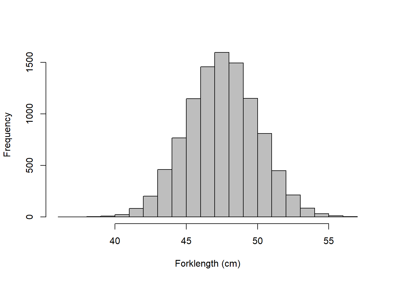
length_sample <- rnorm(n = 10000, mean = x_bar, sd = sigma)

# Plot the sample to see if it is a normal- YAY it is!
hist(length_sample,
  col = "gray",
  main = "",
  xlab = "Forklength (cm)"
)

We’ve add a couple of new arguments to the histogram call to make it a little less ugly here. In Chapter 4 we are going to ramp it up and play with some plots!