18.2 Poisson regression

Poisson regression is useful for situations in which we have a response (independent variable) that is a count. These are discrete data that cannot be considered continuous because it is impossible for them to take on non-integer or non-negative values. Common examples of these types of responses include species count data in ecology, cell or colony counts in biology, and the number of respondents or patients reporting a side-effect or symptom of interest in health care studies.

For the Poisson family, the link function that we will use is the “log” link function. This one is exactly what it sounds like. This link function allows us to work with data that are constrained to be non-negative, a desirable property when we are working with count data.

We will walk through the crabs data set for both the Poisson and negative binomial examples, addressing some distributional assumptions and model fit along the way.

# Read in the data. These data also are available through
# the glm2 package in R.
crabs <- read.csv("data/crabs.csv", header = TRUE)

# Have a look-see
head(crabs)

##   color spine width mass satellites
## 1     2     3  28.3 3.05          8
## 2     3     3  26.0 2.60          4
## 3     3     3  25.6 2.15          0
## 4     4     2  21.0 1.85          0
## 5     2     3  29.0 3.00          1
## 6     1     2  25.0 2.30          3

18.2.1 Data explanation

These data are described in Chapter 13.2. If you need a reminder of what they are go ahead and check them out there.

We are going to convert color to a factor to start because it is currently stored as a numeric variable.

# We want to convert color to
# a factor right off the bat
crabs$color <- as.factor(crabs$color)

Next, we’ll fit a “full” model that assumes the number of satellites is a function of width, mass, spine condition, and color.

# Fit a model
poisson_mod <- stan_glm(
  satellites ~ width + mass + spine + color,
  data = crabs,
  family = poisson()
)

Before we go any further, let’s have a quick look at the model diagnostics using the methods we applied to linear models in Chapter 9. Right away, we can see that this model is not a very good fit to the data.

First, put the fitted.values and the residuals from this stanreg object into a dataframe so we can plot them. I am using the same names that are assigned by glm() so I don’t have to change my code.

resids <- data.frame(.fitted = poisson_mod$fitted.values, 
                     .resid = poisson_mod$residuals)

Now, we can plot them:

ggplot(resids, aes(x = .fitted, y = .resid)) +
  geom_jitter() +
  xlab("Fitted values") +
  ylab(expression(paste(epsilon)))

Just as in the models we fit with glm() in Chapter 13, a few things should jump right out at you from this plot. First, there is some kind of trend happening at the bottom of our plot where the residuals slant downward from left to right. That’s something that should scream “not good!” at you, even if you don’t know why. Second, this plot doesn’t really make it look like our residuals are symmetrically distributed with a mean of zero. But, it is really hard to tell from this graph, especially because of the weird patterns at the bottom of the scatter plot.

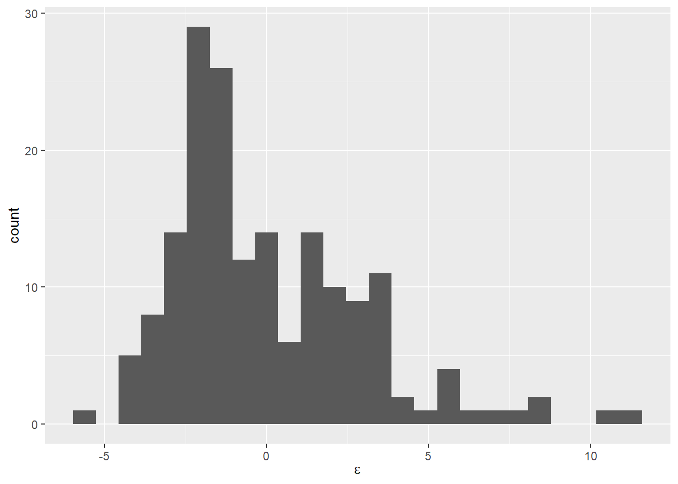
We can check this second concern using a histogram if we want to see if it “looks normal” like this:

ggplot(resids, aes(x = .resid)) +
  geom_histogram(bins = 25) +
  xlab(expression(paste(epsilon)))

Now that we see it presented this way, it is pretty clear that our residuals are not symmetrically distributed around zero even if the mean is about zero. We could also calculate some descriptive statistics for the residuals to really nail this down.

mean(poisson_mod$residuals)

## [1] -0.04047373

Hmmm…the mean is fairly close to zero here, but we’ve already talked about the fact that the mean isn’t a very good descriptive statistic for distributions that we suspect or know are not normal. What about the median as a measure of central tendency?

median(poisson_mod$residuals)

## [1] -0.9278425

Wow, okay, that is a bit more negative than the mean, and at this point we may start to question whether we can say that the residuals are normally distributed with a mean of zero.

So, why has this happened to us? Recall that the Poisson distribution is controlled by a single parameter, \(\lambda\), that is both the mean and the variance of the distribution. If we had started by doing data exploration we would have, of course, noticed that even though the data represent counts, they are pretty clearly over-dispersed (variance is much larger than mean) and are indicative of a negative binomial sampling distribution.

For now, we won’t bother to look at the results or the predictions from this model because the link function is the same for Poisson and negative binomial, so we can get the results from the negative binomial regression in the same way later if that works. Plus, if our model is in violation of assumptions then the results will be unreliable anyway.