16.2 Intro to Bayes Theorem
Bayes Theorem provides the mathematical framework through which Bayesian inference is applied to quantitative questions. The theorem, in the most basic sense, helps us understand the probability of some event given conditions we suspect are related to that event. This elegant theorem was first derived by Reverend Thomas Bayes in the 1700s. The equation was later reworked by Pierre-Simon Laplace to yield the modern version that we use today:
\[P(A|B) = \frac{P(B|A)\cdot P(A)}{P(B)}\]
which is read “the probability of A given B is equal to the probability of B given A times the probability of A, divided by the probability of B”.
A common example application of this theorem that may be of interest to biology students is the probability of having cancer at a given age (thanks Wikipedia!). The example goes something like this:
Suppose we want to know the probability that an individual of age 50 has cancer. We might only have information about the marginal probability of their having cancer given that they are a human (let’s say 1%), and the probability of their being 50 years old given population distribution of ages (let’s just say 3% for the sake of demonstration). To calculate the conditional probability that an individual who is 50 years old has cancer, we would need one more piece of information: the probability that a person with cancer is 50 years old. The calculation is relatively straightforward if we know this number exactly, and we can derive an exact conditional probability. For this example, let’s start by assuming the probability that people who have cancer are 50 years old is 2%. Now we can calculate the conditional probability that a person who is 50 years old has cancer:
Start with the theorem:
\[P(Cancer|Age 50) = \frac{P(Age 50|Cancer)\cdot P(Cancer)}{P(Age 50)}\]
Through substitution we get: \[P(Cancer|Age 50) = \frac{(0.02\cdot 0.01)}{0.03}\]
And now we can solve for the conditional probability: \[P(Cancer|Age 50) = 0.00667\]
Hopefully, you can see from this example and earlier learning about rules of probability why this is such an important theorem in statistical probability theory. In fact, this is one of the reasons for the recent resurgence in the use of Bayes Theorem in applied Bayesian inference in biological and ecological statistics during the past couple of decades. But, if it’s so useful, then why has it only been heavily used recently?
It will quickly become obvious to you that the answer is “computers”. To demonstrate this, let’s consider a slightly more complex example.
Now, let’s assume that we don’t actually have exact information about the probability that individuals who have cancer are age 50. Let’s instead assume that we only have a rough idea about that probability, and that we can put a loose distribution around it. Now, there is no longer an exact mathematical solution for Bayes Theorem but rather an infinite number of potential solutions. If we know the distribution, then we can discretize the distribution and find a finite number of solutions to the theorem that would allow us to describe the probability of our event of interest most of the the time. (This should sound like calculus. Because it is. Don’t worry, you don’t need to do calc here.) However, there are cases for which this problem becomes intractable without the use of computers, even when the distribution is known. You can imagine that this becomes considerably more complex if the form of the distribution is not known with certainty.
For the sake of demonstration, let’s examine how this procedure changes if we have some uncertainty in one of our probabilities on the right-hand side of the equation:
Looking back at our example, we had:
\[P(Cancer|Age 50) = \frac{P(Age 50|Cancer)\cdot P(Cancer)}{P(Age 50)}\]
And, by substitution:
\[P(Cancer|Age 50) = \frac{0.02\cdot 0.01}{0.03}\]
Let’s now assume that the proportion of people with cancer who are also 50 years old is now an unknown quantity that is drawn from a beta distribution that can be described by parameters \(\alpha\) = 200, and \(\beta\) = 10,000:
\[P(Cancer|Age 50) = \frac{Beta(200, 10000) \cdot 0.01}{0.03}\]
Realistically, this is a much tighter distribution than we would use for a situation like this, but we’ll discuss that later. The point is that even a little uncertainty makes the process more complicated than if exact values are known.
We can make this distribution in R:
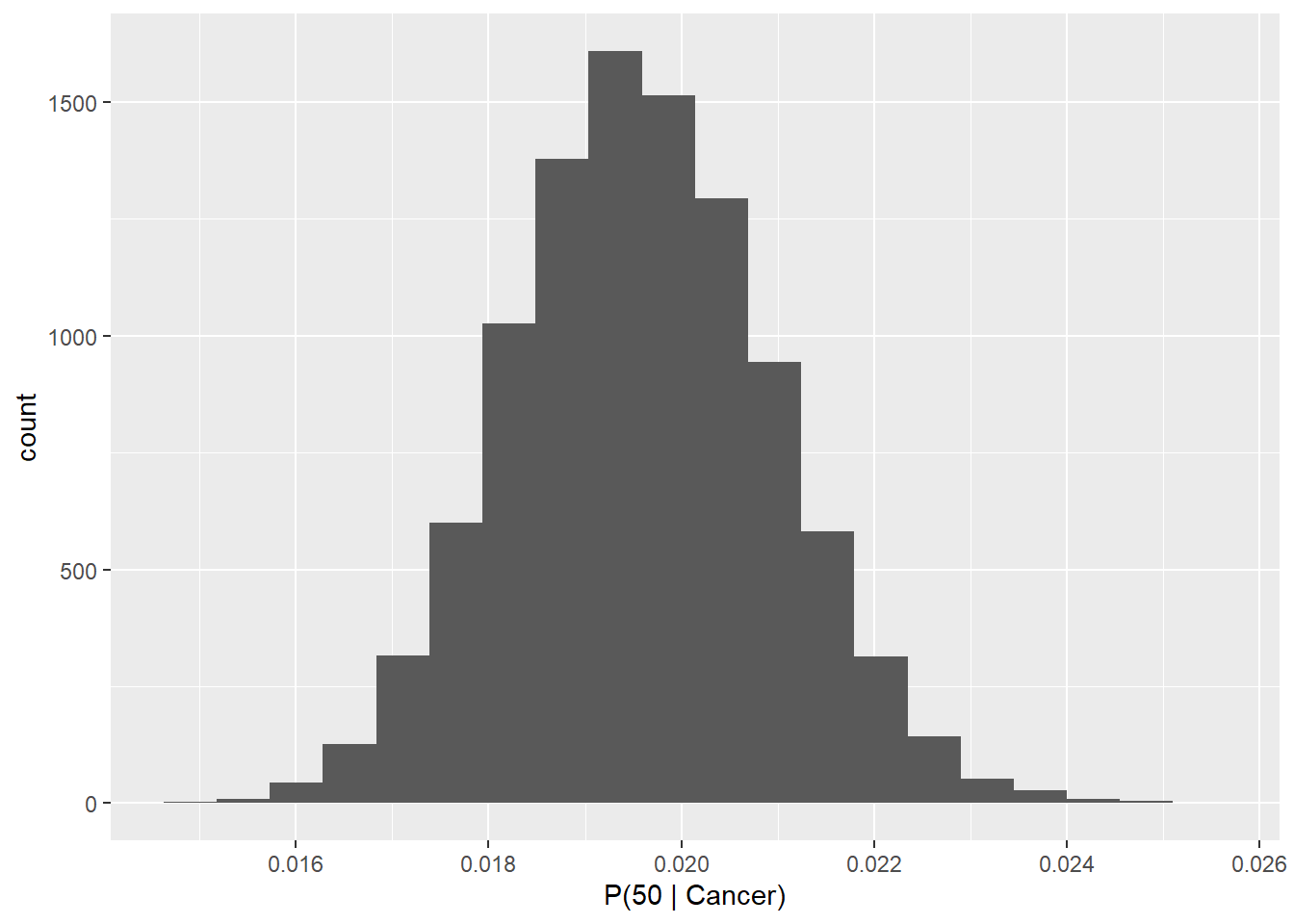
We can also look at this distribution:
# Make the object into a df with
# a single column automatically
# named p_cancer_50
p_50c <- data.frame(p_50_cancer)

# Plot it
ggplot(p_50c, aes(p_50_cancer)) +
  geom_histogram(bins = 20) +
  xlab("P(50 | Cancer)")
Now, we have a working probability distribution for the probability of being age 50 given that one has cancer. We can plug this into Bayes Theorem and construct a probability distribution to solve for the inverse: the probability of having cancer given that the patient is age 50 \((P(Cancer|Age 50))\). Let’s do it in R.
First, let’s define our other marginal probabilities as variables in R.
p_cancer <- 0.01 # Marginal probability of having cancer
p_50 <- 0.03 # Marginal probability of being age 50
Now we can solve the theorem for our finite number of observations:
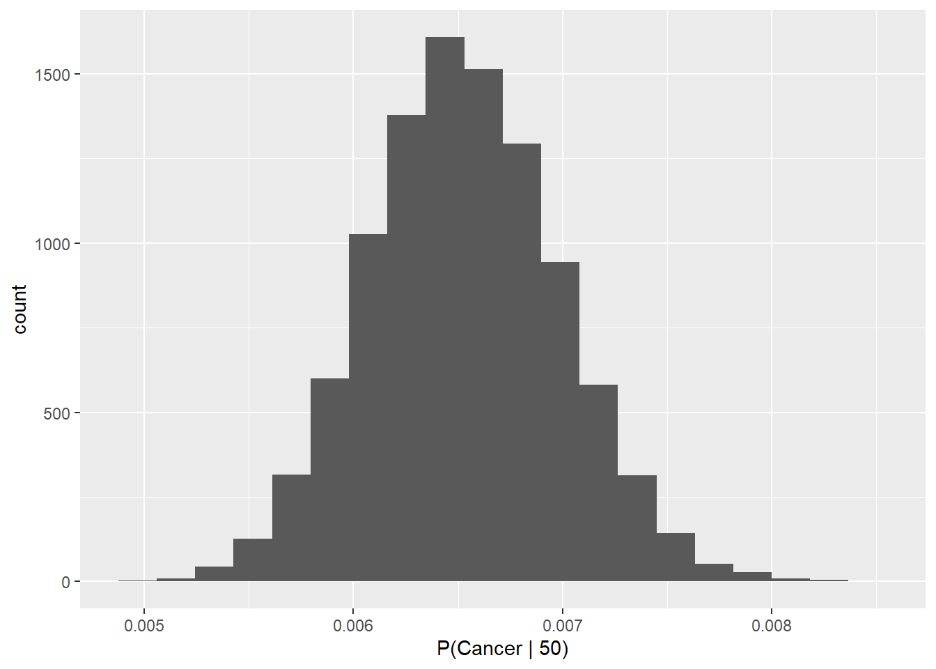
We can calculate descriptive statistics for the conditional probability so that we can describe the distribution.
## [1] 0.006529057## [1] 0.0004550698We can calculate quantiles (95% CRI). Note that in Bayesian inference, we are going to call these ‘credible intervals’ (CRI) or ‘high density intervals’ (HDI) depending on assumptions related to normality, but they are functionally the same thing as ‘confidence intervals’ as far as we are concerned (tell no one I said that eveR).
##        2.5%         50%       97.5%
## 0.005670059 0.006517883 0.007441685
We can also look at the actual distribution:
# Make the object into a df with
# a single column automatically
# named p_cancer_50
p_c50 <- data.frame(p_cancer_50)

# Plot it
ggplot(p_c50, aes(p_cancer_50)) +
  geom_histogram(bins = 20) +
  xlab("P(Cancer | 50)")
Finally, let’s say now that there is uncertainty in all of our probabilities of interest:
# First, let's define each of our
# probabilities as variables in R
p_50_cancer <- rbeta(1e4, 20, 1e3)
p_cancer <- rbeta(1e4, 10, 1e3)
p_50 <- rbeta(1e4, 30, 1e3)
We can continue as before. We solve the theorem for our finite number of observations:
We calculate descriptive statistics for the conditional probability to describe the probability using a mean and standard deviation.
## [1] 0.006858331## [1] 0.002993227Quantiles (95% CRI and median):
##        2.5%         50%       97.5%
## 0.002601671 0.006387833 0.014118524
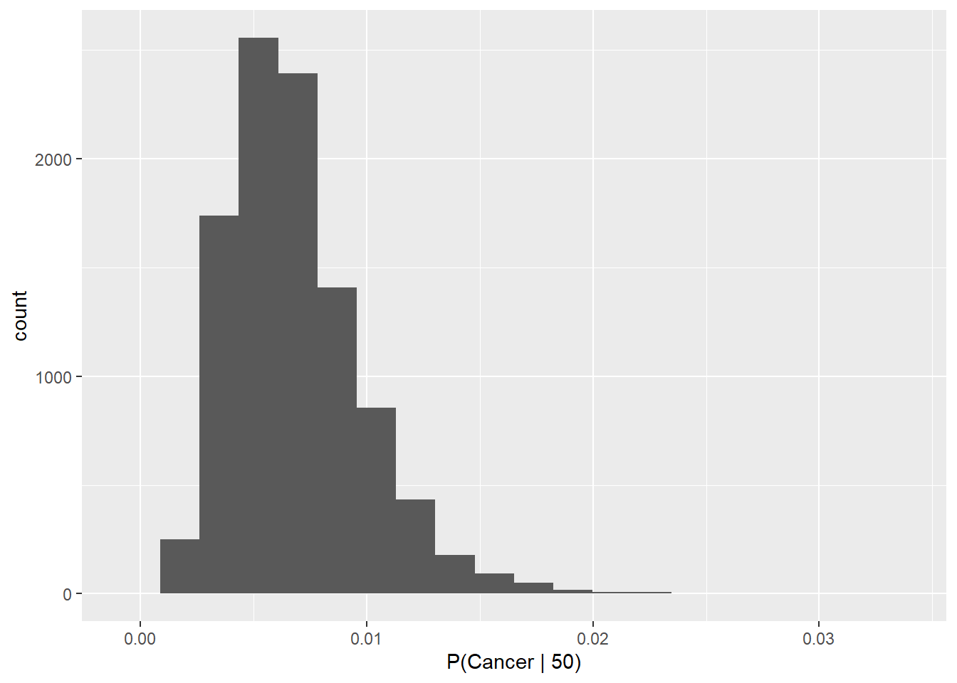
And, have a look at our new distribution:
# Make the object into a df with
# a single column automatically
# named p_cancer_50
p_c50 <- data.frame(p_cancer_50)

# Plot it
ggplot(p_c50, aes(p_cancer_50)) +
  geom_histogram(bins = 20) +
  xlab("P(Cancer | 50)")
Now you can see why computers are starting to matter, and we are not even doing Bayesian inference yet. Why is that?
Because we still haven’t collected any data!!! All that we have done here is state some basic mathematical representations of our beliefs about certain conditional and marginal probabilities of specific events. Those beliefs may be useful representations, or they may be way off!
This mathematical formulation of our ‘beliefs’ is known as the prior distribution for the probability of the event of interest. “Want to know more about the prior distribution”, you say? How convenient…