16.7 More diagnostics
In this section, we will examine some diagnostics to assess the convergence of our parameter estimates and identify any unusual trends in the chains we use for estimation. But, it takes a little while to get there.
First, a brief foray into how these models are estimated. Basically all Bayesian estimation methods rely on some variant of Monte Carlo (random) sampling. Depending on the algorithm, we draw a parameter value, plug it into the model likelihood and evaluate the likelihood of the parameter value relative to the data collected, and then make some decision about whether or not to keep that estimate as part of the posterior distribution (our final parameter estimate). We do this thousands of times, and all of the parameter values that we keep become part of the posterior parameter estimate. We use computer algorithms to determine which parameters values are considered, how they are chosen and whether they should be retained. These algorithms rely on pseudo-random or guided walks called “Markov chains”. Collectively the approach is referred to as Markov Chain Monte Carlo estimation. For each iteration of the model, we retain one value of each parameter for each chain, and we run multiple chains (usually 3-4). We then assess model stability by examining how well the chains mix (\(\hat{r}\)) and whether there are pathological issues related to autocorrelation between samples (n_eff). Stan and other software programs output each value of each parameter for each chain and each run of a Bayesian model. Therefore, instead of just getting a mean and 95% confidence interval, we get thousands of individual estimates that we can use to calculate whatever descriptive statistics or derived quantities we choose (e.g. Difference = post(Group A) - post(Group B)).
16.7.1 Trace plots
In the plot below, the x-axes are model iteration number. Each point on a line shows the parameter value drawn for each chain (of 4 that are run by default) for each iteration that we ran the model (default = 4,000 runs). We can see that there is a high degree of overlap between the four chains, which should inspire some confidence because it means that all of the chains converged on a similar space in each panel (parameter) below.

16.7.2 Colinearity
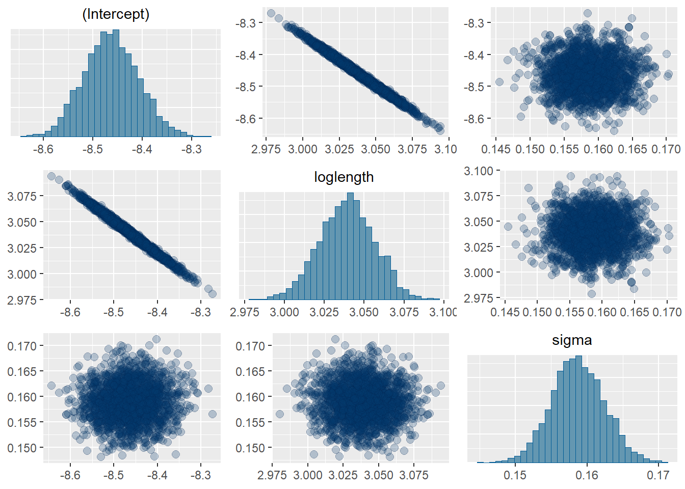
Next, we can take a look at the pairs plot to see whether there are any obvious correlations of concern between our parameters. As anticipated, everything looks okay here, except we do see that we have a pretty strong correlation between our intercept and slope parameters. This is not important for this specific analysis, but we would want to consider this if we were estimating slopes and intercepts independently for each population (site) in the data set.

16.7.3 Divergence
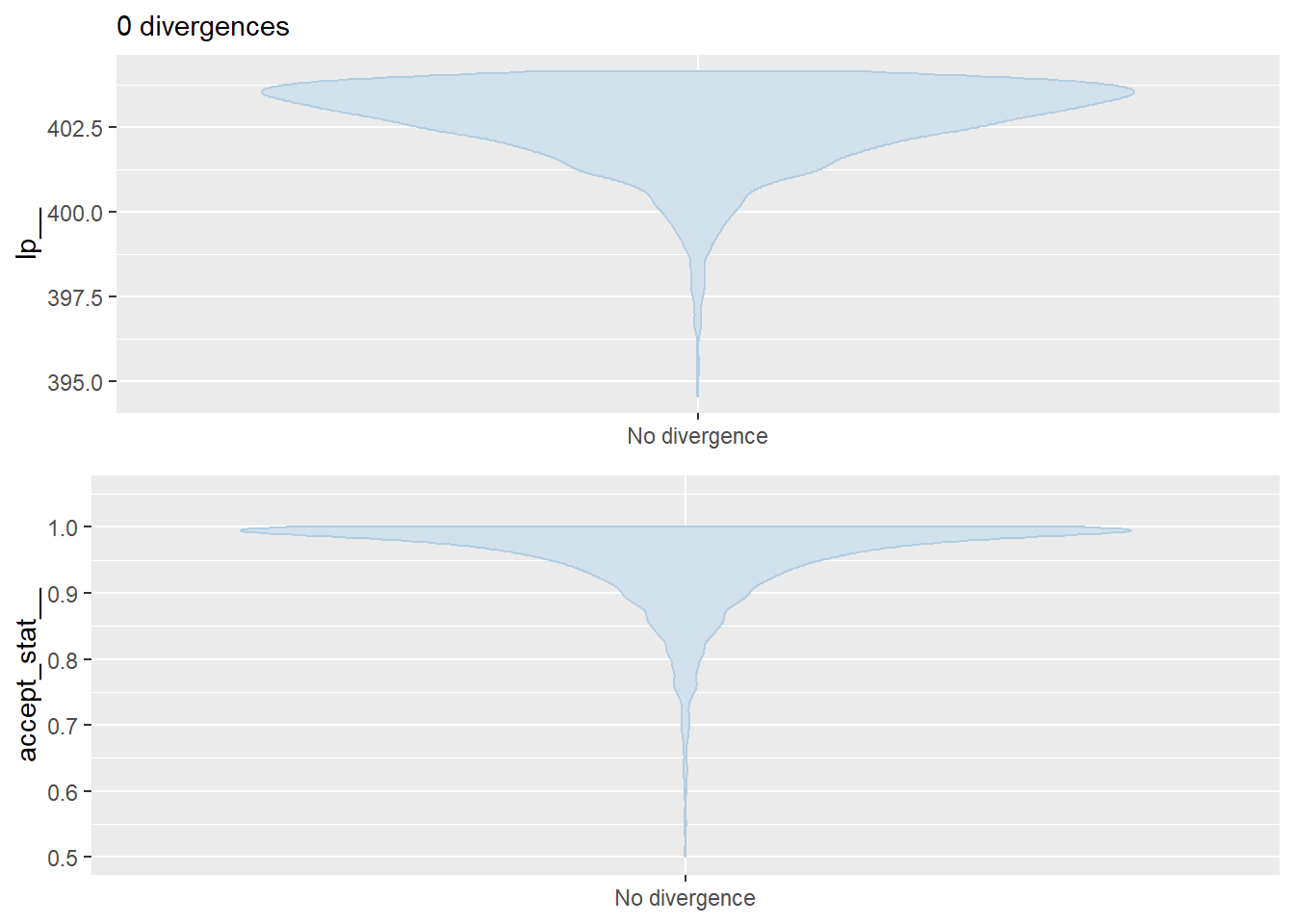
Not like the movies, like “does not follow expectation”. Divergent transitions are an indication that something has gone wrong in your model. You can read more about them here someday, once you understand the first three paragraphs in this section of the Stan Manual [(Chapter 15.5)] (https://mc-stan.org/docs/2_25/reference-manual/divergent-transitions.html). For now, understand that divergence in this sense is a bad thing and it probably means you have a problem with the model that you’ve created. It doesn’t mean you have to throw your data in the garbage. There are some tools in Stan to account for this. But, this is usually a good sign that there is at least something in your model you could change to make it easier to estimate. This could mean changing the likelihood, transforming the data, or re-casting it in another way. Even though that can be scary, we still need to take a look!
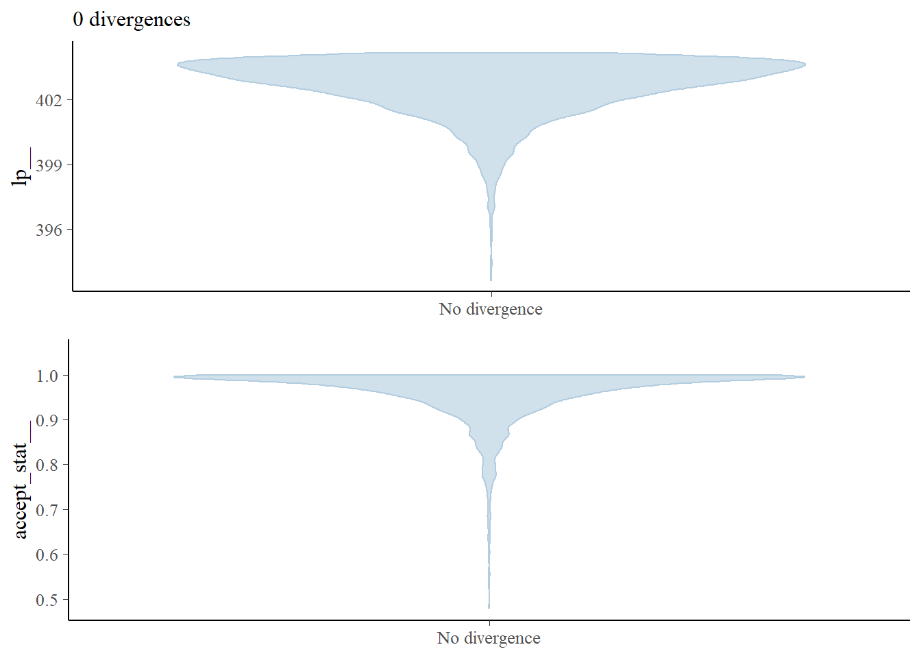
By default, models fit using RStan will throw a warning if there are divergent transitions. You can get a quick of whether or not this is an issue like so:

Again, no problems here as far as we are concerned. We will address any further issues related to divergence as they arise later in the textbook or class.