9.5 Data exploration

9.5.1 Independence of observations

This assumption basically means that each row of your data was collected independently of all others. In other words, no two rows of your data are related to one another.

We can relax this assumption by explicitly including variables and constructs within the models that actually account for these kinds of relationships. For example, in one-way ANOVA we include grouping (factor) variables to to account for non-independence of some observations. In fact, this lack of independence is often the very thing we are interested in testing! In ANOVA, we are interested in whether individuals from the same group respond in the same way. Note that this in turn places the assumption of independence on individual measurements within our groups. It’s turtles all the way down. (I say this a lot. If you don’t know what it means go Google it.)

This assumption really should be be addressed within the context of experimental design. Violations generally require alternatives to the simple cases of one-way ANOVA, ANCOVA or simple linear regression that we will discuss in later chapters. We will discuss specific extensions of our basic linear models (ANOVA and regression) to relax more difficult violations such as repeated observations, and temporal or spatial autocorrelation among observations. Although we can’t cover all of these extensions in one book or a single bottom-up biometry class, we can point you in the right direction for most of them.

You: Get to the point, what are we looking for here?

Me: Sorry. [writes rest of chapter]

For linear models, we want data that were sampled randomly and independently from all other data points. For this information, we have to examine the actual experimental design. In a best case, an experiment is designed intentionally so that all groups get opposite treatments and those there is no correlation (relationship) between treatments (“orthogonal design”). This is easy to achieve with some thought in the design of controlled experiments, but can be difficult or impossible to do in semi-controlled experiments or observational studies. This is one reason why controlled experimentation has long been thought of as the gold standard in science.

There is one obvious thing that is going to tell us that the observations in turtles are not collected independently, but there are a few others. What is it? You can probably infer the answer just from the variable names.

head(turtles, 10)

##             ID Year   Gear Width Removed Status Stay nHooks
## 1       AL-002 2013      J  1.45      UE      1    9      1
## 2  AL-LT14-001 2014      J  6.25      ME      0    4      1
## 3  AL-LT14-003 2014      J  5.45     NaN      1   16      1
## 4  AL-LT14-004 2014  Kahle  2.77       B      0    6      1
## 5  AL-LT14-006 2014      J  4.75      ME      1   49      2
## 6  AL-LT14-006 2014 Circle  2.92     NaN      1   49      2
## 7     LT13-001 2013  Kahle  2.22      ME      1   29      1
## 8     LT13-003 2013      J  1.34      ME      0    4      1
## 9     LT13-004 2013      J  1.63      ME      1   33      1
## 10    LT13-008 2013      J    NA      LE      1   26      2

If you look closely, you’ll notice that we have repeated observations of individuals here. So, we already know that our data do not conform to the assumptions of ANOVA, linear regression, or ANCOVA - but let’s keep using these data for the sake of demonstration. There is, of course another major violation of our assumptions that has to do with experimental design (that is commonly violated): these are discrete data! We’ll pretend for now that we can think of Stay as a continuous variable, though.

You can see how this could get tedious to do for every level of every grouping factor and then for each continuous variable. So, we can also take a “shotgun” approach and look at how variables are related to one another.

This approach allows us to look at relationships between all variables at once. Note below that I am using all columns except ID because that graph would be a mess.

# Look at correlations between variables
pairs(turtles[ , 2:ncol(turtles)])

But, for this data set this is really gross and difficult to interpret due to the nature of the variables. This should tell you that thinking about this stuff before you collect data is really important!

It would make a lot more sense for something like the built-in swiss data because those variables are all continuous. You can check that out by running pairs(swiss) in your code. Look at all of the related variables in the swiss data! This relatedness is called collinearity and can cause some issues if we are not careful about it.

We’ll talk about problems related to correlation between variables (e.g. temperature and photoperiod) in detail when we discuss model selection and collinearity. In the sections that follow, we’ll just focus our efforts on diagnosing Year as a categorical explanatory variable and Width as a continuous explanatory variable.

9.5.2 Normality

In all linear models we make the assumption that the residual error of our model is normally distributed with a mean of zero. This allows us to drop the error term, \(\epsilon\) from computation in the model fitting and allows us to calculate an exact solution in the case of ANOVA and linear regression. (Technological advances have really made this unnecessary because we can solve everything through optimization now).

There are a multitude of tools at our disposal for examining normality of the residuals for linear models. One option is to examine group-specific error structures as a surrogate for residual error prior to analysis. The other option is to examine diagnostic plots of residuals directly from a fitted model object in R or other software programs (this is actually the more appropriate tool).

We are looking to see if the response variable within each group is normally distributed. To assess this, we need to think in terms of the moments of a normal distribution that we learned about earlier in the course, specifically skew and kurtosis. Here we are looking for outliers in the data, or sample distributions that are highly skewed.

First, we could go level by level for all of our grouping variables and conduct Shapiro tests (not shown here).

We can look at a few different plots of our response to start teasing apart some of the potential violations of our assumptions.

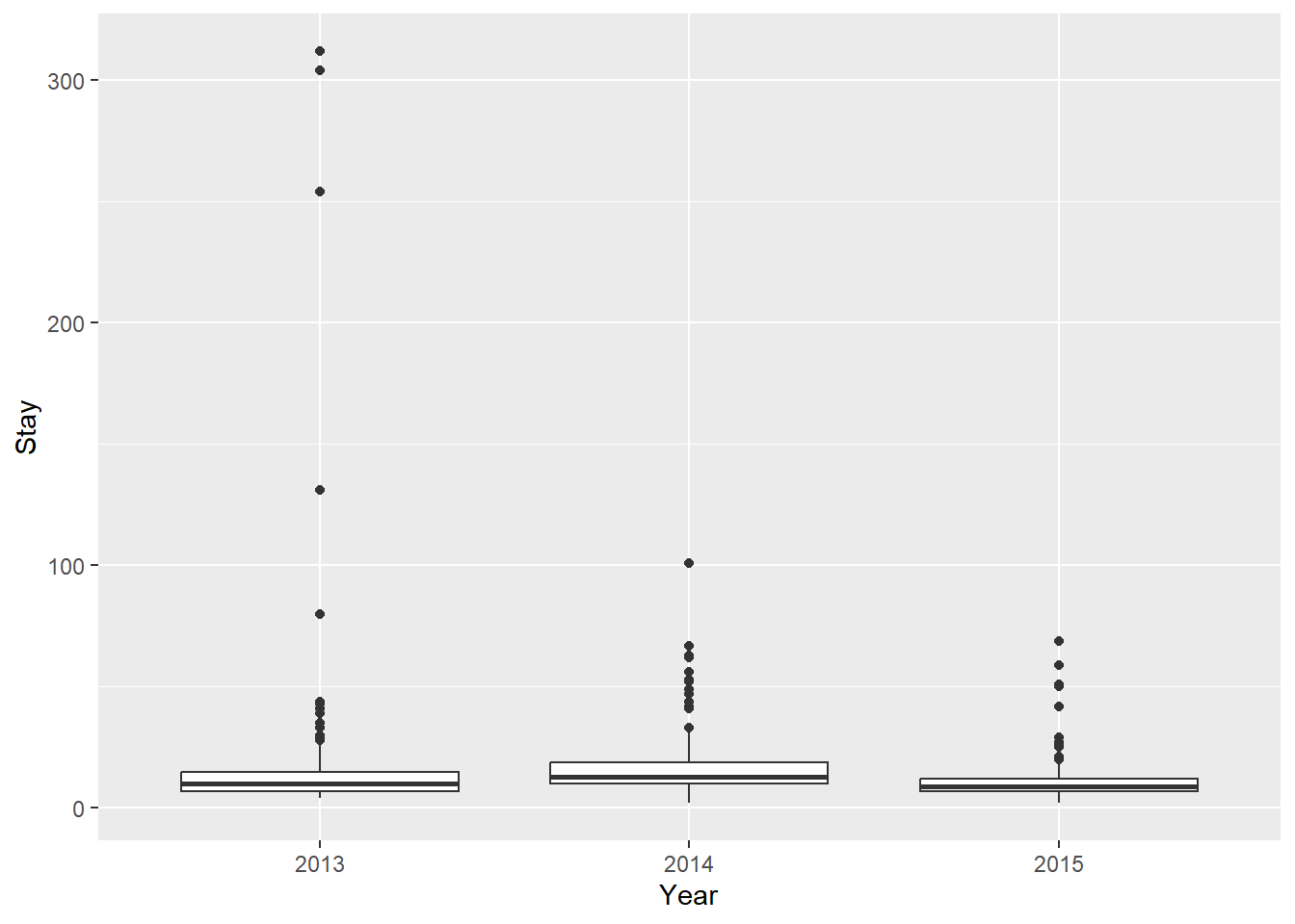
We know we will need to look at a year effect here because that is yet another form of non-independence (and potentially homogeneity) in our data. Let’s start with a boxplot:

ggplot(turtles, 
       aes(x = factor(Year), y = Stay, group = Year), fill = 'gray87') +
  geom_boxplot() +
  xlab("Year")

Whoa! We have a couple of issues here.

First of all: we have clearly identified a number of ‘outliers’ in our data. These are the circles that are outside the whiskers of our box plots.

One way to address these outliers is by dropping them from the data. We only want to do this if we have a pretty good justification for this ahead of time (“a priori”). And, sometimes these can be some of the most interesting observations.

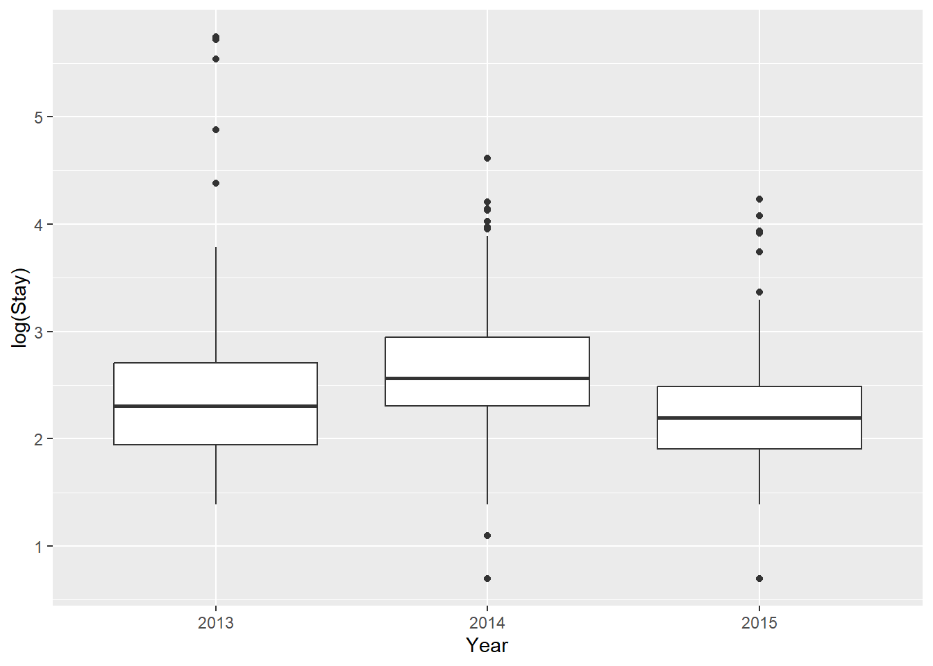
Another way to deal with this is through data transformation. For example, we could use a log transformation in an attempt to normalize extreme values in our data. This certainly looks a little better, but may not get us all the way there…

ggplot(turtles, 
       aes(x = factor(Year), y = log(Stay), group = Year), 
       fill = 'gray87') +
  geom_boxplot() +
  xlab("Year")

NOTE: I will not cover variable transformation extensively in this class or text. The justification is: 1) you can Google it to learn more about what transformations are useful for what, and 2) I will argue that most of the time there are better methods for dealing with non-normal data and then I will show you how to use those methods as we go.

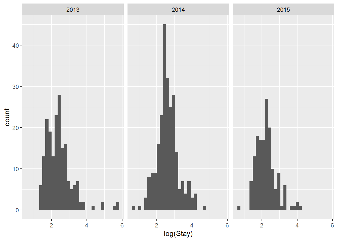
We can also look at histograms to investigate normality within groups. We’ll continue using log(Stay) for now.

ggplot(turtles, aes(x = log(Stay))) +
  geom_histogram() +
  facet_wrap(~ Year)

Again, a little better, but perhaps not as good as we’d like.

9.5.3 Homogeneity of variances

Finally, we assume in all of our linear models that variability in our residuals (which are really just part of our variances) are constant among groups or across the range of continuous variables \(x\). This is the same assumption that we made for t-tests and tested with the F-test in Chapter 6. We’ll now look at a few options for linear models in this chapter depending on how the data are structured.

A quick check of variances in the Stay variable by Year will make it clear that we are also in violation of this assumption if we do not log-transform the data.

turtles %>%
  group_by(Year) %>%
  summarize(var(Stay))

## # A tibble: 3 x 2
##    Year `var(Stay)`
##   <int>       <dbl>
## 1  2013      1435. 
## 2  2014       164. 
## 3  2015        91.7

You can go ahead and conduct a few F-tests if you don’t believe me that these are different, but I’m pretty sure you won’t convince me that the ratios of any two of these variances are equal to 1.00!

This, too, is made magically (A little) better when we log-transform Stay:

turtles %>%
  group_by(Year) %>%
  summarize(var(log(Stay)))

## # A tibble: 3 x 2
##    Year `var(log(Stay))`
##   <int>            <dbl>
## 1  2013            0.556
## 2  2014            0.360
## 3  2015            0.321