11.6 Model validation

Once we have selected a best model, or a set of explanatory variables that we want to consider in our analysis, it is important that we validate that model when possible. In truth, comparison of the validity of multiple models can even be a gold-standard method for model selection in itself (e.g. LOO-IC), but we are not going to go there this semester because it would require a much richer understanding of programming than we can achieve in a week.

Model validation is the use of external data, or subsets of data that we have set aside to assess the predictive ability of our models with data that were not used to estimate the parameters. That is, we can use new data to test how well our model works for making predictions about the phenomenon of interest. Pretty cool, I know!

There are lots of different methods for model validation, most of which use some of your data for fitting (or training) the model and then saves some of the data for predicting new observations based on your model parameters (testing). The most common form of model validation is called cross-validation.

Very generally speaking, there are a large (near-infinite) number of ways to do model validation based on how you split up your data set and how you choose to evaluate predictions. This blog gives a nice overview of these methods with the iris data set in R using the caret package. We’ll write a little code so you can see how it works, though.

11.6.1 Leave-one-out cross validation

We will do some manual cross validation here to demonstrate the general procedure. In order to do that, we will use a “loop” to repeat the process over and over again. For each iteration (i), we will choose a subset of the swiss data to use for training and set the rest aside for comparing to our predictions. Then, we will fit the education model and store the result. Finally, in each iteration, we will store the training data and the predictions in separate lists that we can then use to visualize the results of our model validation. For this example, we will use leave-one-out (LOO) cross validation, but other methods such as “k-fold” that use specified chunks of data are also common. I just prefer LOO, especially because you are likely to run into this one in the near future as it becomes increasingly easy to use and increasingly useful for model comparison via LOO-IC in Bayesian statistics.

First, we need to make a couple of empty vectors to hold our training data and our predictions for each iteration of our cross-validation loop. We define n as the number of rows in the data and will use this as the total number of iterations so that each data point gets left out of the data set exactly once in the process.

# Number of rows in the data set
# Also the number of times the for loop will run
n <- nrow(swiss)

# Will hold observation of Fertility withheld for each iteration
fert_obs <- vector(mode = "numeric", length = n)

# Will hold observation of Education withheld for each iteration
ed_obs <- vector(mode = "numeric", length = n)

# Will hold our prediction for each iteration
fert_pred <- vector(mode = "numeric", length = n)

Now, drop one data point, fit the model, and predict the missing data point one row at a time until you have done them all.

# Repeat this for each row of the data set
# from 1 to n until we have left each row out
for (i in 1:n) {

  # Sample the data, leaving out the ith row
  # These will be our 'training data'
  data_train <- swiss[-i, ]

  # These will be the data we use for prediction
  # We are just dropping the rows that were used for training
  data_pred <- swiss[i, ]

  # Fit the model that tests the effects of Education
  # on the Fertility
  mod_ed <- lm(Fertility ~ Education, data = data_train)

  # Predict Fertility from the fitted model and store it
  # Along with values of Fertility and Education
  fert_obs[i] <- swiss$Fertility[i]
  ed_obs[i] <- swiss$Education[i]
  fert_pred[i] <- predict(mod_ed, data_pred)
}

Let’s put our observed (left-out) data and our predictions for each iteration in a dataframe that we can use for plotting the results of model validation.

loo_df <- data.frame(fert_obs, ed_obs, fert_pred)

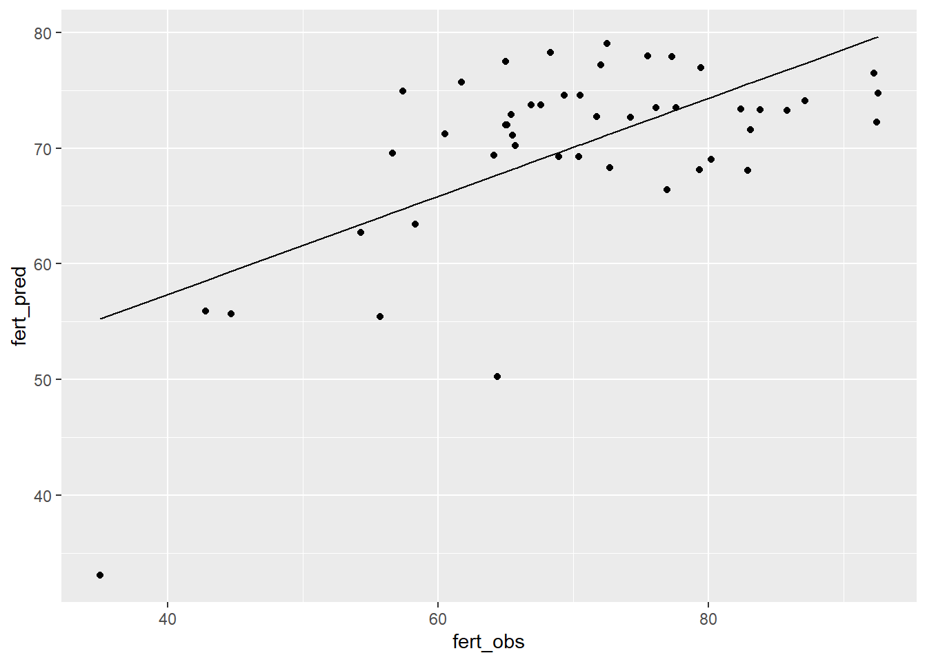
Now, We can look at a plot of our predicted values for each iteration against the data point that was withheld for making the prediction.

ggplot(loo_df, aes(x = fert_obs, y = fert_pred)) +
  geom_point()

We can add a regression line to the plot to see whether we are over or under predicting Fertility from our model in a systematic way:

# Fit the model
pred_line <- lm(fert_pred ~ fert_obs, data = loo_df)

# Make predictions
loo_pred <- predict(pred_line, loo_df)

# Add them to the loo_df
loo_df_pred <- data.frame(loo_df, loo_pred)

# Plot the line against the observed and predicted Fertility
ggplot(loo_df_pred, aes(x = fert_obs, y = fert_pred)) +
  geom_point() +
  geom_line(aes(y = loo_pred))

You can see that we are generally okay, but tend to under-predict at both low and high values of Fertility because the points on either end of the line fall mostly below the line. This is due either to a lack of data at extremes or some overlooked non-linearity in the relationship between X (Education) and Y (Fertility). If we intentionally collected more data at the extremes of Education that could resolve which is the case (because we would either improve prediction at extremes or see the non-linearity in the relationship more clearly). We will use log-transformations to deal help linearize these relationships in some future examples.

We could also look at the summary of our observed vs predicted regression to see how good we are (how much variance in prediction is explained by the model). In this case, it is not great. If we were going to use this for model prediction, we might want there to be a stronger correlation between the observed and predicted values. In that case, it might just mean collecting more or better data or it could mean re-thinking what is being measured and how.

# Extract the R-squared for observed vs predicted
summary(pred_line)$r.squared

## [1] 0.3991715

There are lots of other takes on cross-validation, including popular approaches such as k-fold cross-validation, and a number of simulation-based tools: many of which can be implemented in wrappers available through various R packages. I will leave you to explore these in your leisure time. In general, the more data that are set aside, the more robust the validation is, but we usually don’t want to set aside so much of our data that the training model isn’t representative of the data we’ve collected.

If we are happy enough with our cross-validation results at this point we can go ahead and make predictions from our model.