13.3 Negative binomial regression

Okay, moving on with life, let’s take a look at the negative binomial regression model as an alternative to Poisson regression. Truthfully, this is usually where I start these days, and then I might consider backing down to use of Poisson if all assumptions are actually verified (but, this has literally never happened for me).

We will start this time by actually doing some data exploration before our analysis. This is really how we should have started above, but that would have ruined all the fun.

First, look at the distribution of the data. Here, it should be pretty obvious to you by now that these are count data for which the mean is not equal to the variance…right?

hist(crabs$satellites)

If you think back to a couple of weeks ago, you’ll remember this is a pretty typical example of the negative binomial distribution.

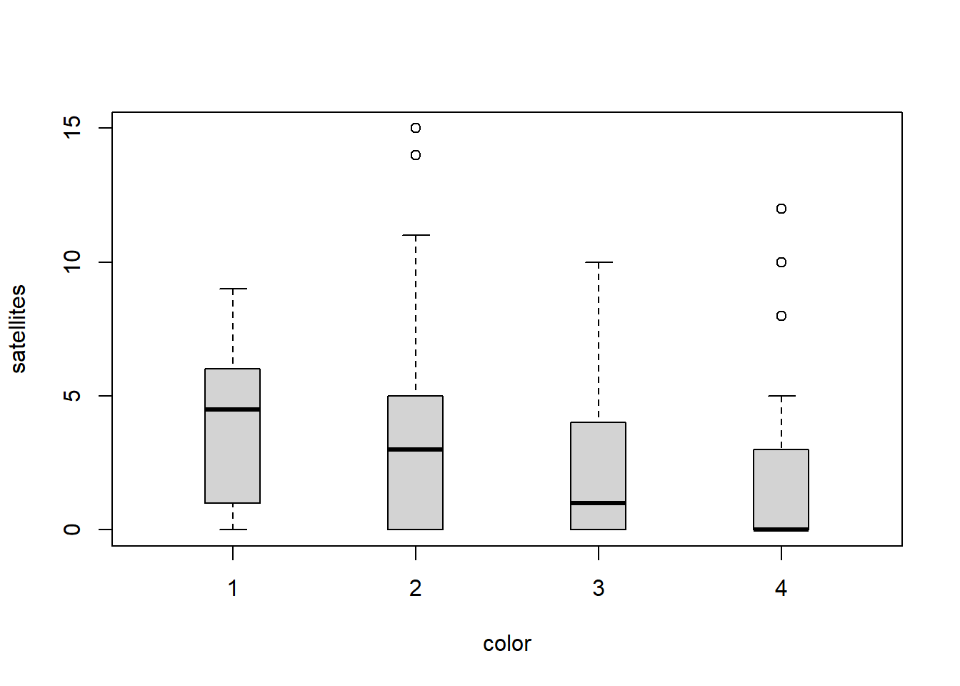
We can take a look at how this shakes out between our groups (color) as well.

boxplot(satellites ~ color, data = crabs, boxwex = 0.3)

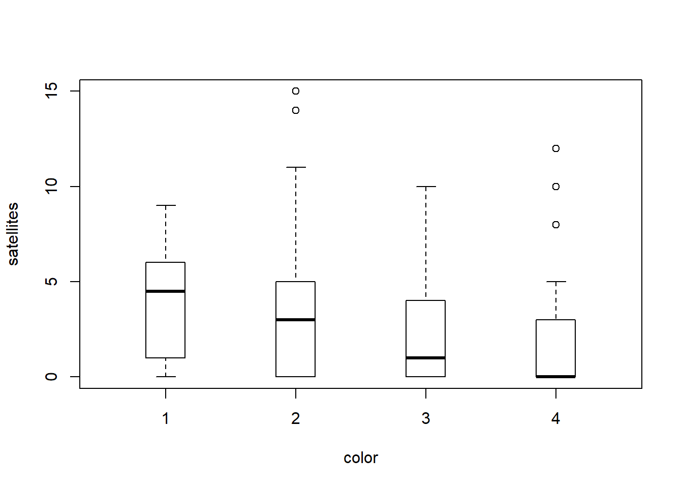
And, you can see here that even within groups the distributions do not look like they are normal or like they have equal variances, so we will fit a GLM that assumes the response is drawn from a negative binomial distribution.

For this example, we will use a function called glm.nb. This function allows us to estimate a GLM for lets us estimate parameters for a GLM that uses the negative binomial error distribution and estimates the “overdispersion parameter” for the negative binomial distribution. You, of course, remember this parameter and know it as theta or size from our discussions about sampling distributions.

We can fit it with the GLM function like this as long as we have the Mass package loaded:

neg_mod <- glm(satellites ~ width + mass + color,
  data = crabs,
  family = "negative.binomial"(theta = 1)
)

Play around with the two formulations above and see if there’s a difference. Clue: there’s not, really. Just two different ways to do the same thing. The functionality in the glm function only came around recently, that’s all.

Now, let’s take a look at the distribution of the residuals. I am going to work with the object I fit using the glm() function. This time, we’ll split our residuals out by color group so we can see where the problems are

ggplot(neg_mod, aes(x = color, y = .resid, fill = factor(color))) +
  geom_violin(alpha = 0.1, trim = FALSE) +
  geom_jitter(aes(color = factor(color)), width = .1) +
  xlab("Fitted values") +
  ylab(expression(paste(epsilon)))

Now we are starting to look a lot more “normal” within groups, and we are getting more symmetrical in our residual sampling distributions. If we had to move forward with this model we could probably do so with a straight face at this point. However, it looks like most of the area of each violin above is below zero (so the mean of our residuals is also negative and non-zero), so we may have some issues going on here that could make this model bad for prediction.

But, how does this compare to the Poisson model for count data? We can use model selection to compare the Poisson model to the negative binomial model, since the response is the same in both cases.

AIC(count_mod, neg_mod)

##           df      AIC
## count_mod  7 919.8796
## neg_mod    6 757.9566

Clearly the negative binomial model is far superior to the Poisson model here. Now, with a reasonable model in hand we could proceed with data visualization, but we might also rather have a “good” model to work with instead of just one that is “good enough”. It turns out that the really problem behind the weirdness in our residuals is actually due to an excess number of zero counts of satellite males on a lot of our females. This is actually really common in count data, where we might observe a lot of zeros before actually counting a success. And, once we have one success (e.g. a parasite infection or illness), we often have extreme events with lots of successes. For example, it might take a while to find a fish with a parasite, or a human with a specific illness, but then that individual could have dozens or hundreds of parasites, or the illness might pop up in a cluster of hundreds of individuals in one location depending on the intensity of the infection. For these cases, we’ll need to deal with the issue these excessive zeros (“zero inflation”) directly.