10.2 Two-way ANOVA
Two-way ANOVA works the same way as one-way ANOVA, except that now we have multiple dummy-coded variables tied up in the intercept. For this example, we will consider a new data set. These data are from an experiment in Restorative Dentistry and Endodontics that was published in 2014. The study examines effects of drying light and resin type on the strength of a bonding resin for teeth.
The full citation for the paper is:
Kim, H-Y. 2014. Statistical notes for clinical researchers: Two-way analysis of variance (ANOVA)-exploring possible interaction between factors. Restorative Dentistry and Endodontics 39(2):143-147.
Here are the data:
10.2.1 Main effects model
We will start by fitting a linear model to the data that tests effects of lights and resin on adhesive strength mpa. Since both lights and resin are categorical, this is a two-way ANOVA. We use the + to imply additive, or main-effects only.
If we make an ANOVA table for this two-way ANOVA, we see that there are significant main effects of resin type but not lights used for drying.
## Analysis of Variance Table
##
## Response: mpa
##           Df Sum Sq Mean Sq F value    Pr(>F)
## lights     1   34.7   34.72  0.6797    0.4123
## resin      3 1999.7  666.57 13.0514 6.036e-07 ***
## Residuals 75 3830.5   51.07
## ---
## Signif. codes:  0 '***' 0.001 '**' 0.01 '*' 0.05 '.' 0.1 ' ' 1
We can also examine the model coefficients for a closer look at what this means.
##
## Call:
## lm(formula = mpa ~ lights + resin, data = dental)
##
## Residuals:
##      Min       1Q   Median       3Q      Max
## -14.1162  -4.9531   0.1188   4.4613  14.4663
##
## Coefficients:
##             Estimate Std. Error t value Pr(>|t|)
## (Intercept)   19.074      1.787  10.676  < 2e-16 ***
## lightsLED     -1.318      1.598  -0.824  0.41229
## resinB         3.815      2.260   1.688  0.09555 .
## resinC         6.740      2.260   2.982  0.00386 **
## resinD        13.660      2.260   6.044 5.39e-08 ***
## ---
## Signif. codes:  0 '***' 0.001 '**' 0.01 '*' 0.05 '.' 0.1 ' ' 1
##
## Residual standard error: 7.147 on 75 degrees of freedom
## Multiple R-squared:  0.3469,	Adjusted R-squared:  0.312
## F-statistic: 9.958 on 4 and 75 DF,  p-value: 1.616e-06
Remember, in our data we had 2 kinds of lights, and 4 kinds of resin. But, here we have one less of each! Why is this? It is because of the way categorical variables are dummy coded for linear models. But, now we have two separate sets of adjustments, so one level of each variable is wrapped up in the estimate for our intercept (lightsHalogen and resinA).
When in doubt, have a look at the model matrix:
##   (Intercept) lightsLED resinB resinC resinD
## 1           1         0      0      0      0
## 2           1         0      0      0      0
## 3           1         0      0      0      0
## 4           1         0      0      0      0
## 5           1         0      0      0      0
## 6           1         0      0      0      0
Right now, you might be a little confused about how to calculate and show the effect size for these variables. If you are not, you should probably take a more advanced stats class and get a better book.
One reasonable option might be to summarize the data by the means and plot the means, but we already decided that we are going to plot our model predictions against the raw data following the form of the statistical model. Rather than go throught the math again, let’s just use the built-in predict() function that I know you now appreciate!
First, we need to do a little magic to get the group combinations for lights and resin into a data.frame that we can use for prediction.
Now we can make our predictions:
dental_y_pred <- predict(
  dental.mod, newdata = groups, interval = "confidence"
  )

pred_dental <- data.frame(groups, dental_y_pred)
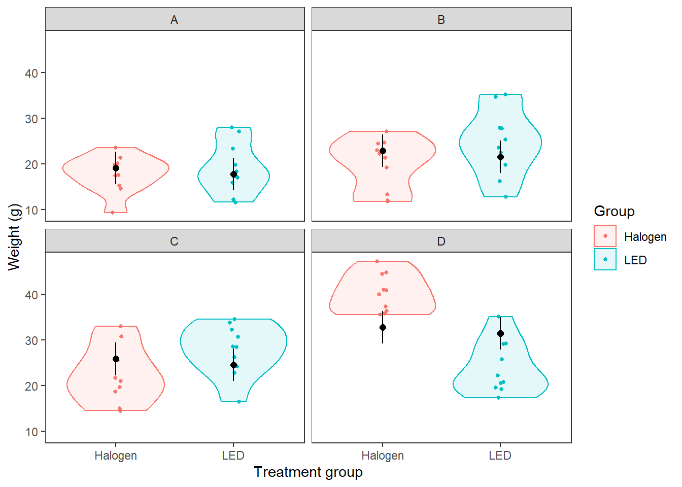
And now we can plot it just like we did for ANOVA:
ggplot(dental, aes(x = lights, y = mpa, color = lights)) +
  geom_violin(aes(fill=lights), alpha = 0.1) +
  geom_jitter(size = 1, width = 0.05) +
  geom_point(mapping = aes(x = lights, y = fit),
             data = pred_dental,
             color = 'black',
             size = 2) +
  geom_segment(
    aes(x = lights, xend = lights, y = lwr, yend = upr),
    data = pred_dental,
    color = 'black') +
  facet_wrap(~resin) +
  theme_bw() +
  theme(panel.grid = element_blank()) +
  xlab("Treatment group") +
  ylab("Weight (g)") +
  labs(fill = "Group", color = "Group")
Now, this looks really nice, but there is definitely something funky going on with Halogen in panel D in the figure above! We have clearly done a poor job of predicting this group. The reason for this, in this case, is because we need to include an interaction term in our model, which makes things even grosser in terms of the math, but is easy to do in R. Of course, if we had been doing a good job of data exploration and residual analysis, we would have noticed this before making predictive plots…
10.2.2 Interactions
To make a model that includes an interaction between lights and resin in the dental data, we will need to go all the way back to our model fitting process.
# The "*" operator is shorthand for what we want to do
# here - more of an "advanced" stats topic
dental_int <- lm(mpa ~ lights * resin, data = dental)
We just have three more columns in our model matrix to distinguish between coefficients for resin that correspond to LED and coefficients for resin that correspond to Halogen. It is at this point that not even I want to do the math by hand!
##   (Intercept) lightsLED resinB resinC resinD lightsLED:resinB lightsLED:resinC
## 1           1         0      0      0      0                0                0
## 2           1         0      0      0      0                0                0
## 3           1         0      0      0      0                0                0
## 4           1         0      0      0      0                0                0
## 5           1         0      0      0      0                0                0
## 6           1         0      0      0      0                0                0
##   lightsLED:resinD
## 1                0
## 2                0
## 3                0
## 4                0
## 5                0
## 6                0
The process for making predictions, thankfully, is identical to two-way ANOVA in R.
Using the groups we made for the main-effects model:
int_y_pred <- predict(
  dental_int, newdata = groups, interval = "confidence"
  )

int_pred <- data.frame(groups, int_y_pred)
And now we plot the predictions against the raw data changing only the name of the data containing our predictions, int_pred.
ggplot(dental, aes(x = lights, y = mpa, color = lights)) +
  geom_violin(aes(fill=lights), alpha = 0.1) +
  geom_jitter(size = 1, width = 0.05) +
  geom_point(mapping = aes(x = lights, y = fit),
             data = int_pred,
             color = 'black',
             size = 2) +
  geom_segment(
    aes(x = lights, xend = lights, y = lwr, yend = upr),
    data = int_pred,
    color = 'black') +
  facet_wrap(~resin) +
  theme_bw() +
  theme(panel.grid = element_blank()) +
  xlab("Treatment group") +
  ylab("Weight (g)") +
  labs(fill = "Group", color = "Group")
You should see below that all of our means match up much better with the observed data in the violins. And, if you go back to the ANOVA output for this model you will see that the interaction term is significant even though lights still is not on it’s own. In coming chapters, we’ll talk about how to design and compare multiple models like these to compare meaningful biological hypotheses against one another.
## Analysis of Variance Table
##
## Response: mpa
##              Df  Sum Sq Mean Sq F value    Pr(>F)
## lights        1   34.72   34.72  1.1067    0.2963
## resin         3 1999.72  666.57 21.2499 5.792e-10 ***
## lights:resin  3 1571.96  523.99 16.7043 2.457e-08 ***
## Residuals    72 2258.52   31.37
## ---
## Signif. codes:  0 '***' 0.001 '**' 0.01 '*' 0.05 '.' 0.1 ' ' 1
Interactions between categorical variables generally are more complicated to deal with than interactions between categorical and continuous variables, because then we are only dealing with straight lines that differ by level. This does not, however, make it any less important for us to communicate how our models fit the observations we have collected. If you can get these tools under your belt, they will be extremely powerful for preparing journal articles, and perhaps more importantly, for communicating your results and the uncertainty surrounding them to stakeholders and public audiences.