20.3 Count models {#20-count}
20.3.1 Data explanation {20-count-data}
We will wrap up our discussions about Bayesian hierarchical GLMs with a worked example of count models. For this one, we will attempt to predict counts of walleye, Sander vitreus, in spawning streams of Otsego Lake, NY, based on historical counts and climate data.
We begin by reading in the data set:
Have a look at the first ten lines of the data set:
And check out the data structure:
## 'data.frame':	71 obs. of  15 variables:
##  $ date     : chr  "2009-04-01" "2009-04-01" "2009-04-01" "2009-04-05" ...
##  $ site     : chr  "Cripple Creek" "Hayden Creek" "Shadow Brook" "Cripple Creek" ...
##  $ counts   : int  1 1 1 4 61 17 50 10 1 35 ...
##  $ high_f   : num  48 48 48 52 52 52 NA NA 39 39 ...
##  $ low_f    : num  34 34 34 32 32 32 NA NA 28 28 ...
##  $ high_c   : num  8.89 8.89 8.89 11.11 11.11 ...
##  $ low_c    : num  1.11 1.11 1.11 0 0 ...
##  $ mean_c   : num  5 5 5 5.56 5.56 ...
##  $ ddPrep   : num  5 5 5 5.56 5.56 ...
##  $ day      : int  91 91 91 95 95 95 97 97 99 99 ...
##  $ year     : int  2009 2009 2009 2009 2009 2009 2009 2009 2009 2009 ...
##  $ dd       : num  72.4 72.4 72.4 109.3 109.3 ...
##  $ dd2      : num  5240 5240 5240 11954 11954 ...
##  $ daylight : num  12.7 12.7 12.7 12.9 12.9 ...
##  $ daylight2: num  161 161 161 166 166 ...
These data are counts of walleye that were captured in spawning tributaries of Otsego Lake during the 2009, 2013, 2017,and 2018 spawning season. These measurements are accompanied by various environmental indicators that include high and low flows, precipitation (rain and snow), high, low, mean temperatures (c) and degree days (dd), and photoperiod (daylight) on each day of the year.
We will use the data to predict number of walleye we expect to see each day in the spawning tributaries based on historical counts and some explanatory variables of interest.
20.3.2 Data analysis {#20-count-analysis}
We start by estimating a model using the stan_glmer() function. Let’s say for the sake of argument that we are simply interested in the lake-wide mean of our counts so that we know when students should, for example, be heading out to tributaries to look for walleyes in streams.
For now, we will model walleye count as a function of photoperiod, with a random effect of site on the intercepts. This model assumes that there is variability in counts of spawning individuals between sites, but that the relationship between photoperiod and count is the same across all sites. In this case, we will specify a quadratic relationship between counts and dates because we expect the number of fish to increase to some point in the run before it decreases. We are not interested in the individual sites in this case, but need to account for repeated observations within spawning locations.
As we look through these results, we can see that we have a significant effect of degree days on spawning behavior. What’s more is that our count of spawning fish appears to increase during the year to a point before it starts to decrease.
But we’ve got what appear to be some major issues related to convergence at the bottom of this output! [dun, dun, dun]
Before we get started, we need to standardize the covariate (dd) as discussed in Chapter 15.3. This helps keep things on a unit scale for model estimation, and prevents wacky estimates like negative variances (!). You can think of this as calculating z-scores for each observation of a given variable.
And now we can fit the model. In the rstanarm package, the model might look something like this:
20.3.3 Predictions {#20-count-preds}
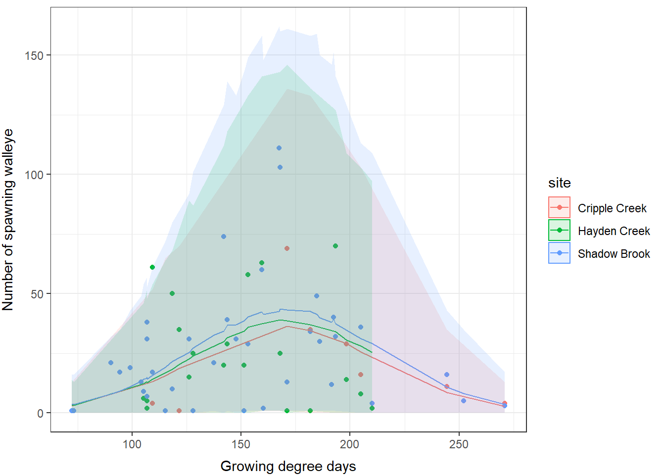
Now, if we want, we can make a graph to show these predictions. Here, we make predictions for all years, and plot by site.
Now, calculate the descriptive statistics and combine with the original data for plotting:
fit <- apply(pred_matrix, 2, mean)
lwr <- apply(pred_matrix, 2, quantile, 0.025)
upr <- apply(pred_matrix, 2, quantile, 0.975)

wae_preds <- data.frame(eyes, fit, lwr, upr)
And we plot the predictions:
ggplot(wae_preds, aes(x = dd, y = counts, color = site, fill = site)) +
  geom_point() +
  geom_line(aes(y = fit)) +
  geom_ribbon(aes(xmin = dd, ymin = lwr, ymax = upr, color = NULL),
              alpha = 0.15) +
  xlab("Growing degree days") +
  ylab("Number of spawning walleye") +
  theme_bw() +
  theme(
    axis.title.x = element_text(vjust = -1),
    axis.title.y = element_text(vjust = 3)
) 
We can see that these estimates are pretty similar to the predictions from the lme4 fit in Chapter 15, but the upper bounds on our credible limits have come down substantially and our predictions now align better with the observed patterns.