5.5 Discrete distributions
Discrete probability distributions are useful for situations in which our random variable of interest can only take specific values within the interval of interest. For example, this might include age, counts, pass/fail, or any number of conceivable categories. As a result, these require a slightly different treatment of probability as a discrete, rather than continuous phenomenon. (Think back to our histogram that we started with in this chapter.)
5.5.1 Bernoulli
The Bernoulli distribution is a special case of the binomial distribution with a single trial (see below for clarification). Bernoulli outcomes are those for which the variable we are measuring can take on one of two values: a one or a zero. This distribution is useful for visualizing processes such as coin flips, yes/no responses, live/dead endpoints in lab studies, and a number of other very interesting phenomena. The Bernoulli distribution has a single parameter: the probability of success, but the number of successful outcomes is also governed by sample size: n, which R calls size because n was already taken.
We can simulate data from a Bernoulli distribution in one of two ways in R.
The “old-school” way of doing this was to draw from a binomial with a single trial. Here we randomly draw a single sample from a binomial with a single trial, and a 50% chance of success. We’ll use the example of hatching chicken eggs with some probability of success. If you are boring, you can think about flipping coins, too!
We’ll start with one chicken egg that has a 50% chance of successfully hatching (probability of success = 0.50).
## [1] 0There is also a function called rbern in the Rlab package that simplifies this for the specific case of a Bernoulli.
Let’s do it again with that function:
## [1] 0Or we could hatch a whole bunch of eggs:
## [1] 1 0 1 0 1 0 1 1 1 0Then, we could even count how many of those were successful. Do you remember how to do that? There are several different ways. You’ll have to come up with one for the homework assignment (hint: see Chapter 2).
5.5.2 Binomial
The binomial distribution is pretty similar to the Bernoulli distribution. In fact, the Bernoulli is just a special kind of binomial. The binomial includes a parameter called \(N\) (size in R) which corresponds to a number of trials per sample. We assume that this is 1 in the case of Bernoulli. In most cases in biology, it will suffice to use the Bernoulli, but for modeling we will want to understand the binomial for things like random stratified designs and nested models that rely on the use of binomial distribution. Later in your career, you might even get into cool models that estimate \(N\) as a latent state to estimate population size (for example). Plus, using the binomial is way faster and can be more precise for certain regression applications [okay, that one should probably have a citation, but this is The Worst Stats Text eveR, so go Google it].
To sample data from a binomial distribution, we can use rbinom from base R. In this example we tell R that we want 10 samples (n) from a binomial distribution that has 10 trials (size) and a probability of success (prob) of 0.5. This is like hatching ten eggs from each of ten chickens instead of just one chicken laying ten eggs.
# Take a random draw of 10 samples
# from a binomial distribution with 10 trials
# and probability of success equal to 0.50
rbinom(n=10, size=10, prob=0.5)
## [1] 5 6 5 6 5 6 4 6 5 3Remember as you look through these that your numbers should look different than mine (at least most of the time) because these are being generated randomly.
5.5.3 Multinomial
The multinomial distribution is a further generalization of the Binomial and Bernoulli distributions. Here, there are one or more possible categorical outcomes (states), and the probability of each one occurring is specified individually but all of them must sum to one. The categories are, in this case, assumed to be a mutually exclusive and exhaustive set of possible outcomes.
We can use the multinomial distribution to randomly sample from categories (imagine our response variable is a categorical variable, like the names of the students in this class).
To do this, we need to read in the s_names.csv file from our data folder that is definitely in your working directory (remember to set your working directory first).
Read in the data file with stringsAsFactors = FALSE for purposes of demonstrating with categorical variables (not factors).
Next, let’s assign the variable name in s_names to a vector for simplicity.
Then, we can assign a uniform probability of drawing any given name if we divide one by the number of names.
# Calculate probability of getting a given
# name based on the length of the vector
prob_each <- 1 / length(name)

# Repeat this probability for each
# name in our vector of names
probs <- rep(prob_each, times = length(name))
probs
## [1] 0.03846154 0.03846154 0.03846154 0.03846154 0.03846154 0.03846154
## [7] 0.03846154 0.03846154 0.03846154 0.03846154 0.03846154 0.03846154
## [13] 0.03846154 0.03846154 0.03846154 0.03846154 0.03846154 0.03846154
## [19] 0.03846154 0.03846154 0.03846154 0.03846154 0.03846154 0.03846154
## [25] 0.03846154 0.03846154This shows us that the probability of drawing any of the individual names is {r prob_each}.
Now, we can sample from a multinomial distribution using our objects. Here we are taking 5 samples from the distribution, each time we sample there is only one trial, and we are sampling with the 26 probabilities above.
Have a look:
##       [,1] [,2] [,3] [,4] [,5]
##  [1,]    1    0    0    0    0
##  [2,]    0    0    0    0    0
##  [3,]    0    0    0    0    0
##  [4,]    0    0    0    0    0
##  [5,]    0    0    0    0    0
##  [6,]    0    0    0    0    0
##  [7,]    0    0    0    0    0
##  [8,]    0    0    0    0    0
##  [9,]    0    0    0    0    0
## [10,]    0    0    0    0    0
## [11,]    0    0    0    0    0
## [12,]    0    0    0    0    0
## [13,]    0    0    0    0    0
## [14,]    0    0    0    0    0
## [15,]    0    0    0    0    0
## [16,]    0    0    0    1    0
## [17,]    0    0    0    0    0
## [18,]    0    0    0    0    0
## [19,]    0    0    0    0    0
## [20,]    0    0    0    0    0
## [21,]    0    1    0    0    0
## [22,]    0    0    0    0    0
## [23,]    0    0    0    0    0
## [24,]    0    0    0    0    0
## [25,]    0    0    1    0    0
## [26,]    0    0    0    0    1
WHOA a matrix??!!! What does it all mean?
Take a step back, breathe, and think about this. The rows in this matrix are you and your classmates. If we took one random sample from the multinomial distribution, it would look like this:
##       [,1]
##  [1,]    0
##  [2,]    0
##  [3,]    0
##  [4,]    0
##  [5,]    0
##  [6,]    0
##  [7,]    1
##  [8,]    0
##  [9,]    0
## [10,]    0
## [11,]    0
## [12,]    0
## [13,]    0
## [14,]    0
## [15,]    0
## [16,]    0
## [17,]    0
## [18,]    0
## [19,]    0
## [20,]    0
## [21,]    0
## [22,]    0
## [23,]    0
## [24,]    0
## [25,]    0
## [26,]    0
Here, we pulled a single sample from the distribution, and probability of sampling a given individual was 0.04 (1/26). If it makes it easier, we can put your names next to it:
##       name
##  [1,] "Ava"         "0"
##  [2,] "Dillon"      "0"
##  [3,] "Delaney"     "0"
##  [4,] "Manolo"      "0"
##  [5,] "Sarah"       "1"
##  [6,] "Shannon"     "0"
##  [7,] "Olivia"      "0"
##  [8,] "Ebony"       "0"
##  [9,] "Julia"       "0"
## [10,] "Davi"        "0"
## [11,] "Gabrielle"   "0"
## [12,] "Jordan"      "0"
## [13,] "Tayler"      "0"
## [14,] "Summer"      "0"
## [15,] "Leah"        "0"
## [16,] "Christine"   "0"
## [17,] "Ashley"      "0"
## [18,] "Katherine"   "0"
## [19,] "James"       "0"
## [20,] "Emily"       "0"
## [21,] "Cassidy"     "0"
## [22,] "Maximillion" "0"
## [23,] "Sierra"      "0"
## [24,] "Kyle"        "0"
## [25,] "Diana"       "0"
## [26,] "Amanda"      "0"
Now, if I was calling on you randomly in class, after 10 questions, the spread of people who would have participated in class might look like this (or whatever you got - remember, it is random):
##       name
##  [1,] "Ava"         "0" "0" "0" "0" "0" "0" "0" "0" "0" "0"
##  [2,] "Dillon"      "0" "0" "0" "0" "0" "0" "0" "0" "0" "0"
##  [3,] "Delaney"     "0" "0" "0" "0" "0" "0" "0" "0" "0" "0"
##  [4,] "Manolo"      "0" "0" "0" "0" "0" "0" "0" "0" "0" "0"
##  [5,] "Sarah"       "0" "0" "0" "0" "0" "0" "0" "0" "0" "0"
##  [6,] "Shannon"     "0" "0" "0" "0" "0" "0" "0" "0" "0" "0"
##  [7,] "Olivia"      "0" "0" "0" "0" "0" "1" "0" "0" "0" "0"
##  [8,] "Ebony"       "0" "0" "0" "0" "0" "0" "0" "0" "0" "0"
##  [9,] "Julia"       "0" "0" "1" "0" "0" "0" "0" "0" "0" "0"
## [10,] "Davi"        "0" "0" "0" "0" "0" "0" "0" "0" "0" "1"
## [11,] "Gabrielle"   "0" "0" "0" "1" "0" "0" "0" "0" "0" "0"
## [12,] "Jordan"      "0" "0" "0" "0" "0" "0" "0" "0" "0" "0"
## [13,] "Tayler"      "0" "0" "0" "0" "0" "0" "0" "0" "0" "0"
## [14,] "Summer"      "0" "0" "0" "0" "0" "0" "0" "0" "0" "0"
## [15,] "Leah"        "0" "0" "0" "0" "0" "0" "0" "0" "0" "0"
## [16,] "Christine"   "0" "0" "0" "0" "0" "0" "0" "1" "0" "0"
## [17,] "Ashley"      "0" "0" "0" "0" "0" "0" "0" "0" "0" "0"
## [18,] "Katherine"   "0" "1" "0" "0" "0" "0" "0" "0" "0" "0"
## [19,] "James"       "0" "0" "0" "0" "0" "0" "0" "0" "0" "0"
## [20,] "Emily"       "1" "0" "0" "0" "0" "0" "0" "0" "0" "0"
## [21,] "Cassidy"     "0" "0" "0" "0" "1" "0" "0" "0" "0" "0"
## [22,] "Maximillion" "0" "0" "0" "0" "0" "0" "0" "0" "0" "0"
## [23,] "Sierra"      "0" "0" "0" "0" "0" "0" "0" "0" "0" "0"
## [24,] "Kyle"        "0" "0" "0" "0" "0" "0" "1" "0" "1" "0"
## [25,] "Diana"       "0" "0" "0" "0" "0" "0" "0" "0" "0" "0"
## [26,] "Amanda"      "0" "0" "0" "0" "0" "0" "0" "0" "0" "0"
Taking this one step further, we could just draw a name and stop looking at these ugly (no but really they are awesome!) matrices:
## [1] "Sierra"And now we have a way to randomly select an individual based on a multinomial distribution. What fun!
5.5.4 Poisson
The Poisson distribution is used for counts or other integer data. This distribution is widely used (and just as widely misused!) for its ability to account for a large number of biological and ecological processes in the models that we will discuss this semester. The Poisson distribution has a single parameter, \(\lambda\), which is both the mean and the variance of the distribution. So, despite its utility, the distribution is relatively inflexible with respect to shape and spread. Fun fact: this distribution was made widely known by a Russian economist to predict the number of soldiers who were accidentally killed from being kicked by horses in the Prussian army each year. It is named, however, after French mathematician Siméon Denis Poisson. [fails to provide citations for any of this]
Take a look at how the distribution changes when you change \(\lambda\), and you will get an idea of how this one works. It is probably the most straightforward of any we’ve considered.
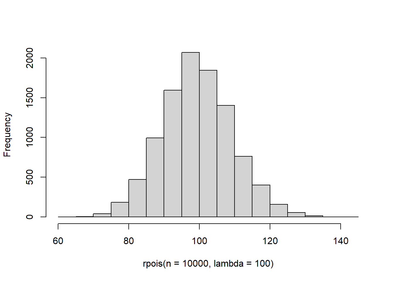
We’ll set it aside for now because it often fails us (or our data fail it, I suppose).
5.5.5 The negative binomial distribution
Okay, this one can be a little difficult to wrap your head around but it’s an important one for us to know about. So, we will spend a little extra time setting this one up to try and be clear. Often, folks start out thinking that they’re going to use a Poisson distribution and they end up collecting with data that do not conform to the relative inflexibility of that single-parameter distribution. Where they end up usually tends to be a negative binomial in a best case (we’ll talk about challenges associated with lots of zeros later in the book).
For the purpose of this class, we are not going to dive into the mechanics of the negative binomial distribution, but we do need to know what it looks like and why we might need it.
One useful way to conceptualize the negative binomial is “how long does it take for some event to occur?” For example, we might ask how long it takes a fish to start migrating, how long it takes a sea turtle to recover in a rehabilitation center, how long it will take for a terminal patient to expire (ooh, that’s dark), or how frequently we see the expression of a gene of interest. These kinds of questions are asked in aptly named “time-to-event” models that rely on the variance structure of the negative binomial. In the context of these kinds of questions, the negative binomial is a discrete probability distribution (and not a continuous distribution) because the “time” component of the distribution is actually a series of independent Bernoulli trials (holy crap!). For example: if we want to know how many days it will take for a turtle to recover from an injury, what we are really doing is asking on each day until recovery, “Is today the day?”. Then, we flip a coin and find out. So, each day in this example is a Bernoulli trial. Another way to think about this is the number of failures occurring in a sequence before a target number of sucesses is achieved.
For the classical parameterization:
We will start by looking at how many failures are observed before one success in a sequence of Bernoulli trials.
With probability of succes equal to 0.95, it doesn’t take long and most of the probability mass is near zero, with a couple of stragglers further out.
# Take a random sample from the negative binomial
Value <- rnbinom(1e4, size=1, prob=.95)

# Make a histogram of it with ggplot
ggplot() + geom_histogram( aes(x = Value) )
If we decrease probability of success in each trial to 0.25, we see more failures on average before we reach success. Most of the time, it still takes less than 5 trials to reach a success, but some times it takes much longer.
# Take a random sample from the negative binomial
Value <- rnbinom(1e4, size=1, prob=.25)

# Make a histogram of it with ggplot
ggplot() + geom_histogram( aes(x = Value) )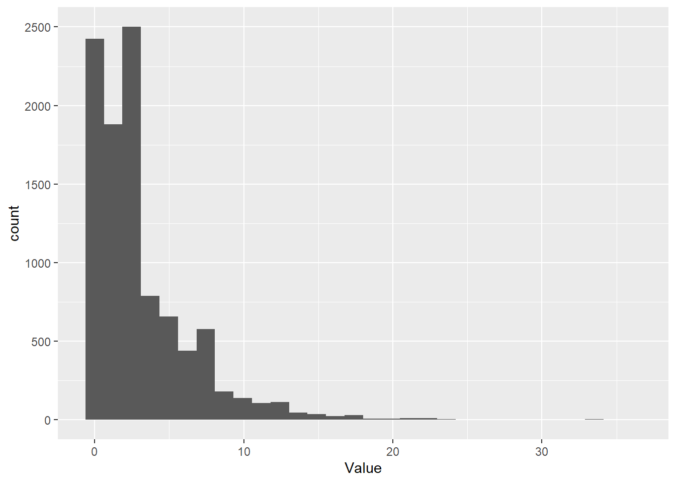
And, if we increase the number of successes that we use for our criterion, or target, then it spreads the distribution out even further.
# Take a random sample from the negative binomial
Value <- rnbinom(1e4, size=10, prob=.25)

# Make a histogram of it with ggplot
ggplot() + geom_histogram( aes(x = Value) )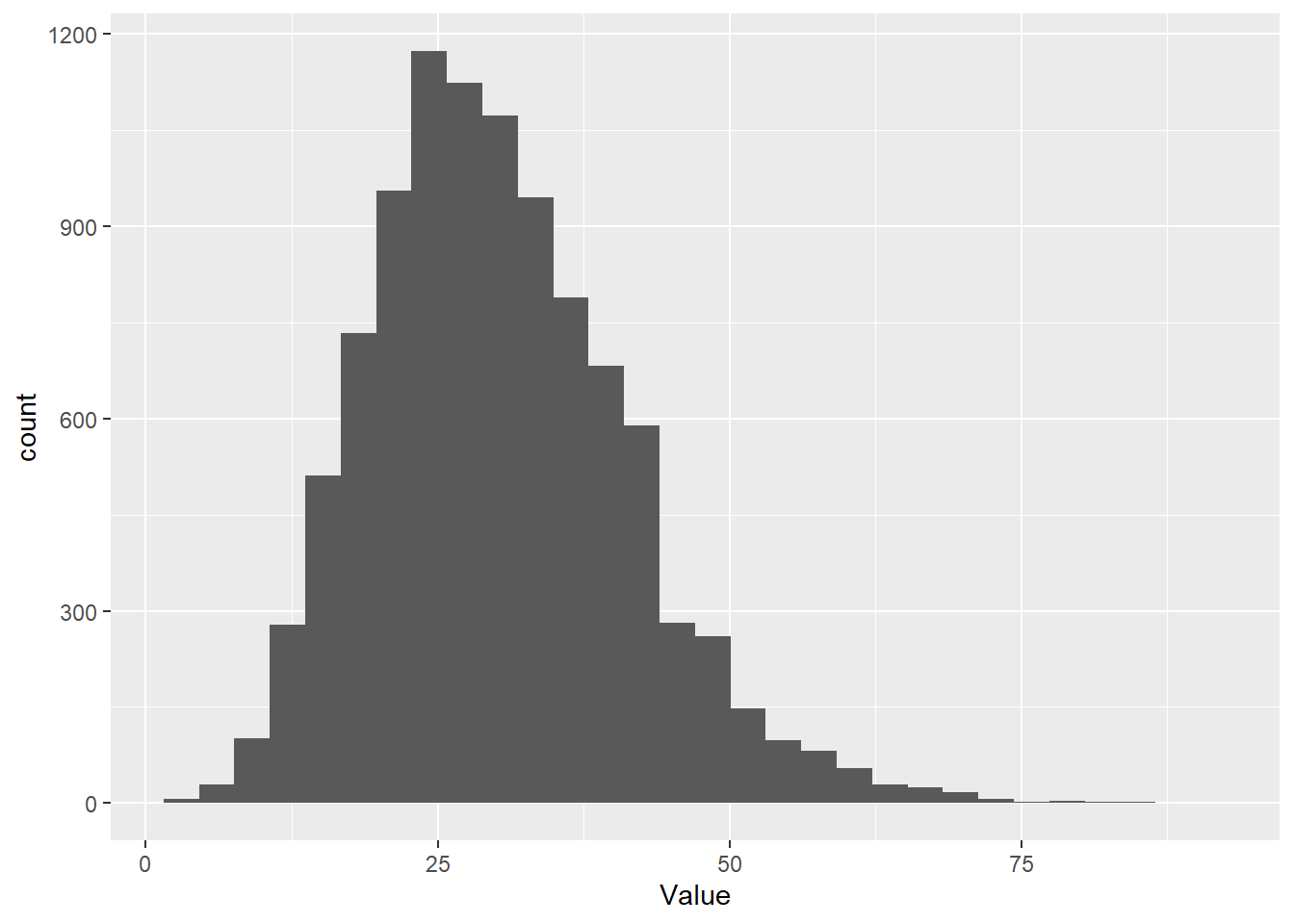
Now, because of it’s properties, the negative binomial is also useful for number of other applications that have nothing to do with interpretting the results of repeated binomial trials. Specifically, it has been widely used to represent Poisson-like processes in which the mean and variance are not equal (e.g., overdispersion). This has seen a lot of application in the field of ecology, especially for overdispersed count data.
Here, we draw 10,000 random samples from a negative binomial distribution with a mean of 10 and an overdispersion parameter of 1. The overdispersion parameter is called ‘size’ because this is an alternative parameterization that is just making use of the relationships between existing parameters of the negative binomial. It’s easy to grasp how the mean changes the location of the distribution.
# Take a random sample from the negative binomial
Value <- rnbinom(1e4, mu = 10, size = 1)

# Make a histogram of it with ggplot
ggplot() + geom_histogram( aes(x = Value), bins = 20 )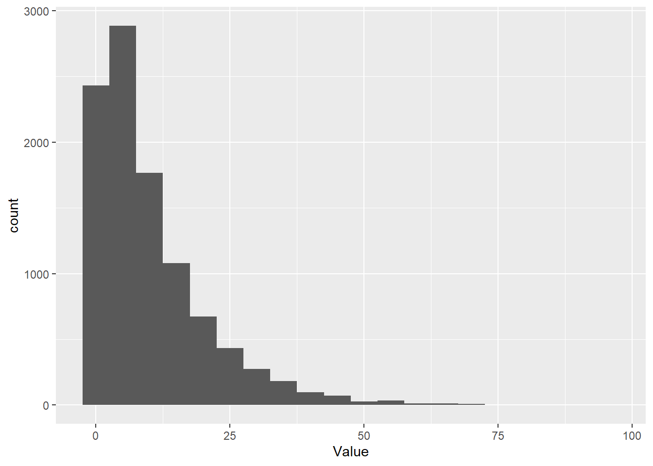
But, note how the overdispersion parameter changes things if you run the following code:
# Take a random sample from the negative binomial
Value <- rnbinom(1e4, mu = 10, size = 1000)

# Make a histogram of it with ggplot
ggplot() + geom_histogram( aes(x = Value), bins = 20 )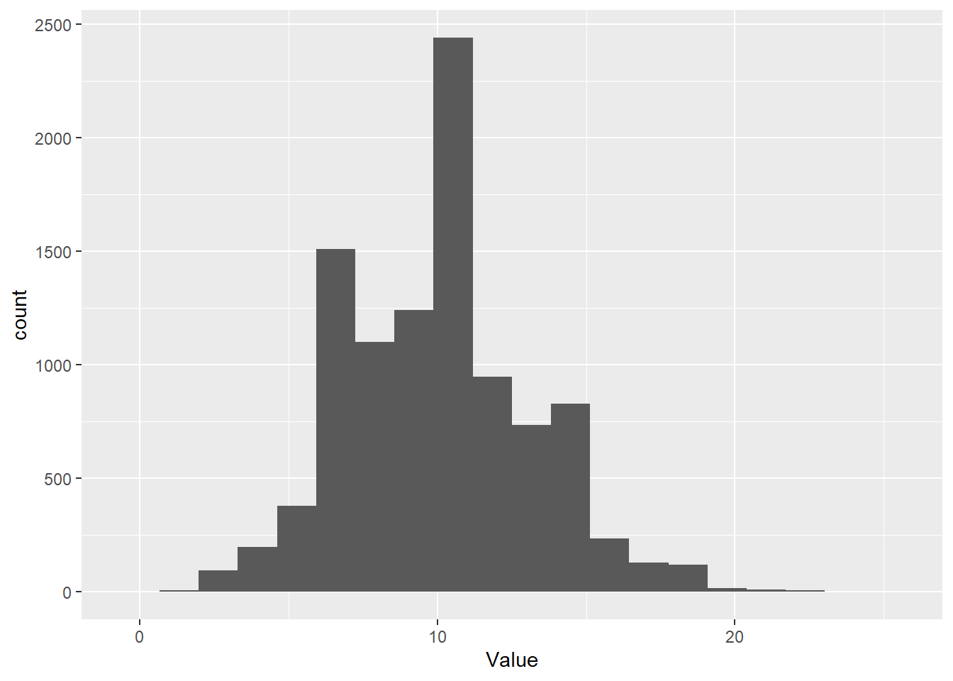
A more intuitive way (I think) to work with the negative binomial in R is by using the MASS package. In this parameterization, we use the mean and the
dispersion parameter explicitly so it makes more sense:
# Take a random sample from the negative binomial
Value <- rnegbin(1e4, mu = 10, theta = 1000)

# Make a histogram of it with ggplot
ggplot() + geom_histogram( aes(x = Value), bins = 20 )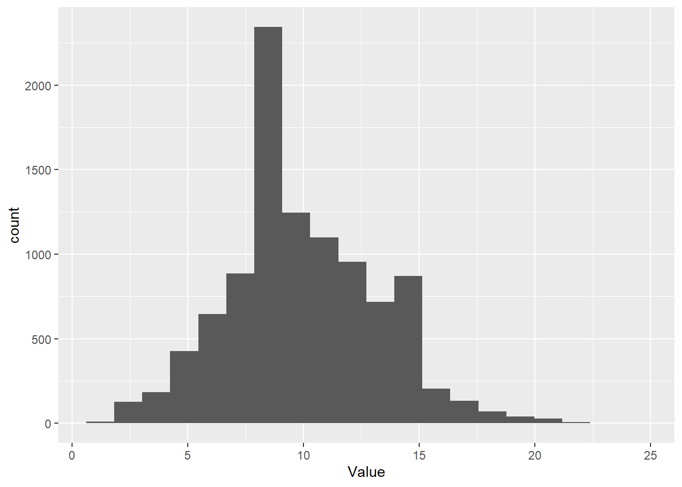
The results are pretty much identical. Just two different naming systems for the parameters.