Dissolved oxygen isopleths
Date manipulation
# First, we convert the date column
# to a character string. We pass the
# result directly to the as.Date
# function, and along with that we
# specify a format so R knows where it
# is looking for specific elements of
# the date info we are trying to pass.
otsego$date <- as.Date(
  as.character(otsego$date),
  format = "%m/%d/%Y"
)

# Remove NA values to make life easier
lim <- na.omit(otsego)

# Multiply depth column by -1 so depth will
# plot from top to bottom.
lim$depth <- -1 * lim$depthIsopleth creation
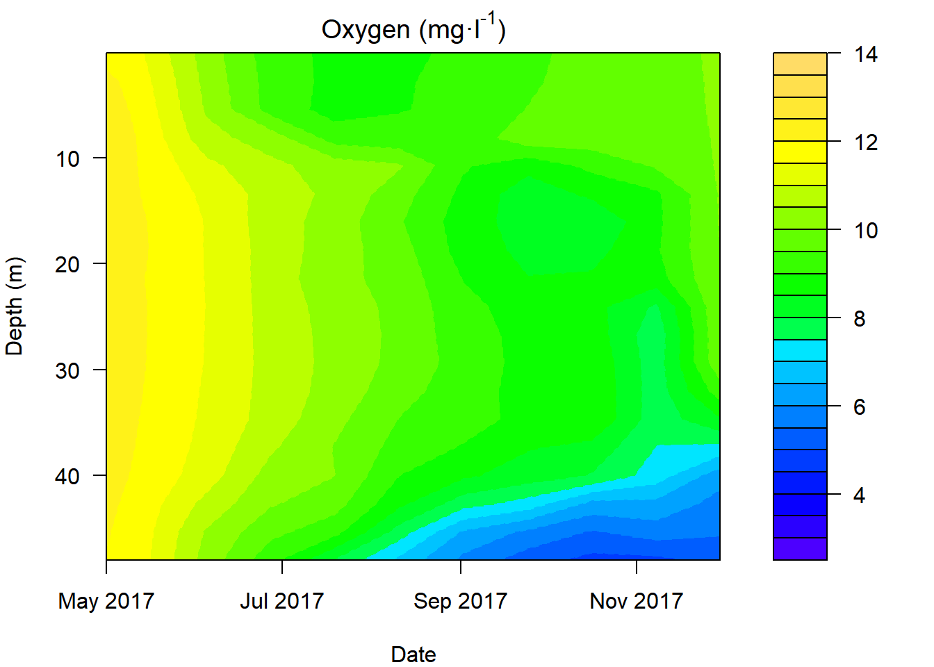
We interpolate do_mgl across date and depth. The interpolation we are using is basically just a bunch of linear regresions to predict do_mgl for values of date and depth across a regular grid. Then, we make the plot.
# Create a data frame containing the
# x, y, and z variables of interest
plotter <- data.frame(x = lim$date, y = lim$depth, z = lim$do_mgl)

# Sort it so we have ascending values of x and y
plotter <- plotter[with(plotter, order(x, y)), ]

# Make a regularly spaced x, y, z grid using
# linear interpolation from the akima package
im <- with(
  plotter,
  interp(x, y, z,
    duplicate = "mean",
    nx = length(unique(lim$date)),
    ny = length(unique(lim$depth))
  )
)

# Plot the isopleth

# Set up plotting window margins
par(mar = c(4, 4, 2, 8))

# Make the graph
filled.contour(
  im$x, # Variable on x-axis (date)
  im$y, # Variable on y-axis (depth)
  im$z, # Response (wq parameter)
  col = topo.colors(26),
  main = expression(paste("Oxygen (mg", "\u00b7", "l"^"-1", ")")),
  # Specify y-axis limits.
  ylim = c(min(im$y), max(im$y)),
  # Specify x-axis limits. In
  # this case, we are "zooming in"
  # on year 2017
  xlim = c(as.Date("2017/05/01"), max(im$x)),
  # X-axis label
  xlab = "Date",
  # Y-axis label
  ylab = "Depth (m)",
  # Axis options
  plot.axes = {
    # This is how we include
    # countour lines
    contour(
      im$x,
      im$y,
      im$z,
      nlevels = 26,
      drawlabels = FALSE,
      col = topo.colors(26),
      lwd = 1,
      lty = 2,
      add = TRUE
    )
    # Y-axis
    axis(2,
      at = seq(0, -50, -10),
      labels = seq(0, 50, 10)
    )
    # X-axis
    axis(1,
      at = seq(as.Date("2017/05/01"),
        by = "2 months",
        length.out = 16
      ),
      labels = format(
        seq(as.Date("2017/05/01"),
          by = "2 months",
          length.out = 16
        ),
        "%b %Y"
      )
    )
  }
)
This work is licensed under a Creative Commons Attribution 4.0 International License. Data are provided for educational purposes only unless otherwise noted.